9. Tutorials¶

This section aims to provide easy and stepping tutorials.

9.1. Tutorial #1¶

To get a primer to ESonix, nothing better than a fast & easy tutorial. This will help you to get the main concepts.

Introduction¶

We will run a really basic layout made of three equal volumes (v1, v2 and v3) connected by two passive vents (cf. Fig. 9.1)

We will simulate an explosion in volume 1.

Main assumptions:

Internal pressure: \(1\ bar\)
Ambient pressure: \(0.2\ bar\)
Discharge Coefficients: \(CD=0.5\)

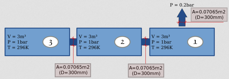
Fig. 9.1 Aircraft Layout

Create the model¶

Step 1: Download the model template¶

A decompression model is a simple Excel spreadsheet. You can start from a blank one although we advice to download a template from our site. You have an easy access from the menu bar, as shown in Fig. 9.2).

Fig. 9.2 Download Template

Save it on your own disk. You can (and you should) rename it. Let’s call it “ESonix_tuto_1.xlsx”.

Step 2: Define the Volumes¶

Edit the file with any Excel-compatible tool, and select the tab “Volumes”.

Fill in the first row with The First Volume (the one on the right on the previous schema) data, i.e:

id: 1
volume: 3
label: “Volume 1”
deck: 0
sta: 1
rbl: 0

Now, go ahead with the two last volumes. Expected tab is shown Fig. 9.3.

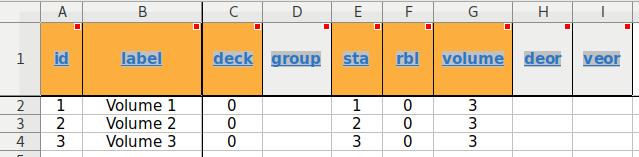
Fig. 9.3 Volumes Definition

The only differences between the rows shown Fig. 9.3 are (apart the labels) the sta values. We put here some dummy values that describe the geometric positions of each volumes.

Columns deck, sta and rbl need a bit of explanations: their values have no impact on calculations results. They are actually used only for post-processing stuff like organising results into relevant sections or drawing A/C layout in a comprehensive way.

By using our template, you will have access to basic data control (try to enter some text in the volume columns). Additionally, some useful data are provided via tool tips.

Now the next step is to define the connections.

Step 3: Define the Connections¶

This is usually the most tricky part, although it will go smoothly for our current example. First select the tab “Connections”.

As defined in Fig. 9.1, we have two connections in this model. Let’s define them as:

Connection #1: Passive vent between Volume 1 and Volume 2, area=0.07065m², Cd=0.5
Connection #2: Passive vent between Volume 2 and Volume 3, area=0.07065m², Cd=0.5

Note

in the Tab “Connections” and Tab “Load_Cases”, the column header of the discharge coefficient is labelled “cp” and not “cd” and stands for the same parameter.

A “passive vent” is called passive by opposition to “featured vent” or “active vent”. A “passive vent” is a simple opening that is always opened , like Toe-kick grids.

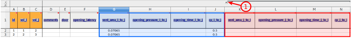
Fig. 9.4 Connections Definition

Note

Observe in Fig. 9.4 how we filled only the relevant fields. The “*_i_to_j” columns (highlighted in Blue in the ESonix Model template) will be interpreted to be zero when empty. ESonix will therefore assume that opening time is \(0\ sec.\) and opening pressure is \(0\ psi\): the connection is always opened for any pressure.

The “*_j_to_i” parameters are highlighted in Red in the ESonix Model template, and can be folded / unfolded with the button (item #1 on Fig. 9.4).

We will actually let them as they are since ESonix will assume that values are the same than “*_i_to_j” values. Here come two major tips:

Any Empty value in the i_to_j columns will be interpreted as “zero”. This is called initialisation phase.
Any Empty value in the j_to_i columns will be internally copied from the i_to_j value. This is called symmetrization phase.

Step 4: Define the Load Cases¶

The last modifications we will perform on our model is to define the so-called load cases. A load case in the decompression process is an opening from the cabin to the ambient.

The tab used for this purpose is titled “Load_Cases”

What defines a load case in last resort is therefore:

Where is the hole opening? Which volume will be connected to the Ambient?
Which size the opening hole is?
Which discharge Coefficient to use?
Which conditions in the cabin (Pressure and Temperature)
Which conditions in the ambient (Pressure)

The answers to this questions are given by the regulations (e.g FAR 25.365e for the opening holes)

For our tutorial, we will create a single dummy load case:

Opening in Volume 1 with a size equal to internal vents. A discharge Coefficient of 0.5 will be used. Pressure in the cabin is \(1\ bar\) whereas pressure in the ambient will be taken equal to \(0.2\ bar\).

Model you should get is shown Fig. 9.5.

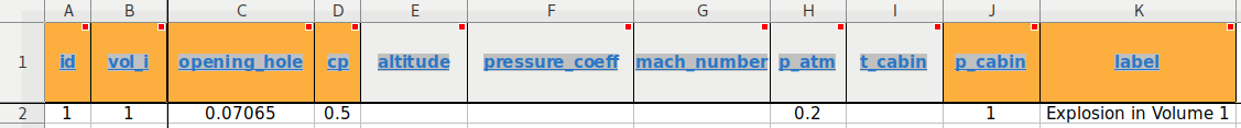
Fig. 9.5 load cases Definition

And that’s it for our model! The next step will consist in creating a new Project on the ESonix platform.

Run your model¶

If you do not have any account on ESonix, it’s time now to create it!

If you are not logged in, well, it’s also time to do it.

Step 5: Create a project¶

Once identified on the platform, create a new project from the top bar (cf. Creating a project).

Fill in the form. Call the project “tuto1” (Fig. 9.6)

Modify default values as follows:

Set Name as “Tuto 1”
Set A/C family as “generic”
Set A/C type as “generic”

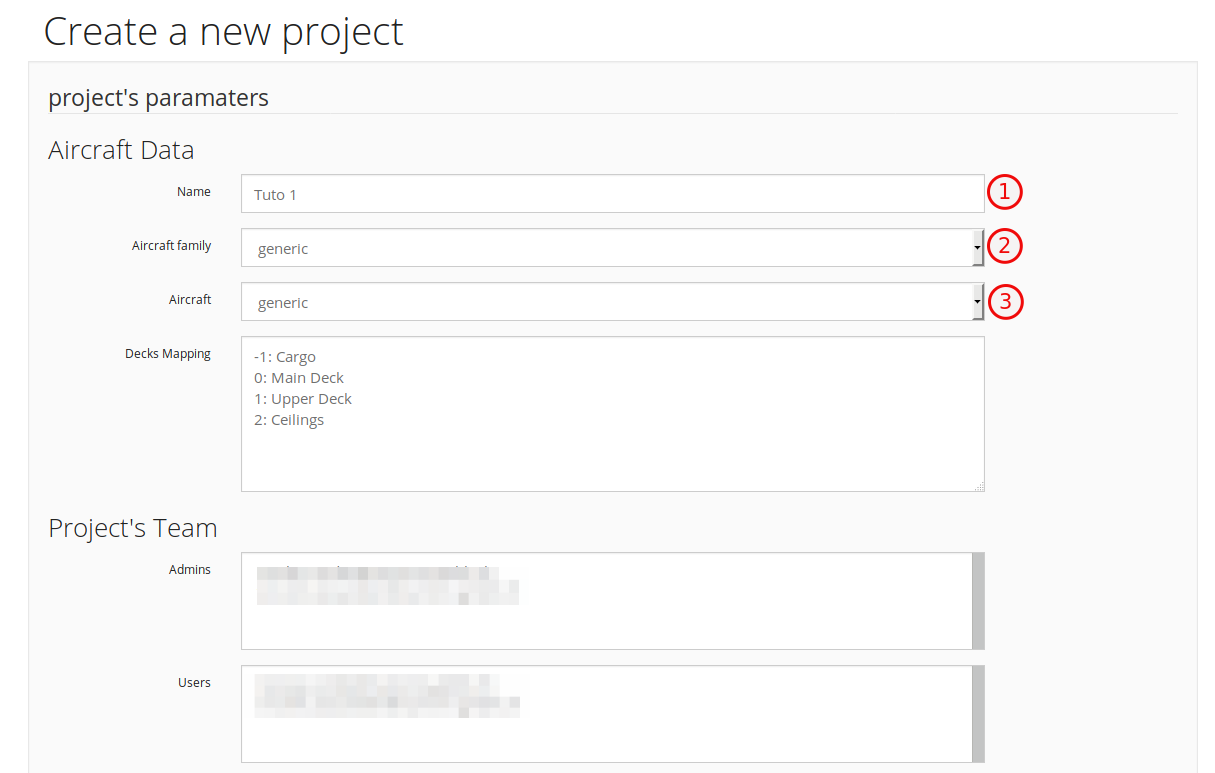
Fig. 9.6 Project Definition

Note

The A/C type field should normally content the Aircraft type, like A319 or B777.

Modify default values as follows:

Set units to “bar, m, Kg”, such as Esonix is aware about how is described the model
Set doors configuration to “Closed”

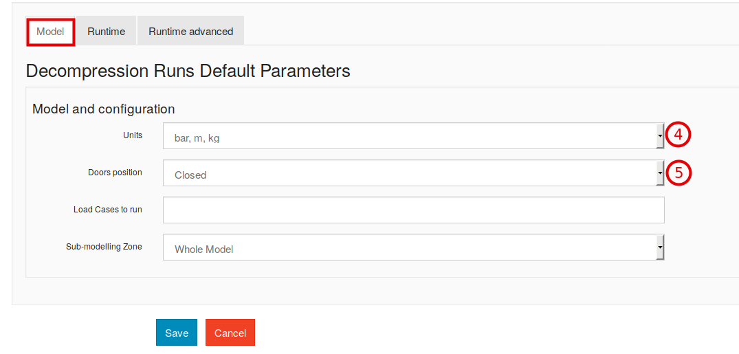
Fig. 9.7 Project Definition (continuation)

Note

For the current tutorial, Doors position actually doesn’t matter since we do not have doors in the model. You may have chosen “Opened”, it wouldn’t have changed the calculations. “Opened and Closed” is useful for real-life models with actual doors installed where we need to simulate both configurations.

Modify default values as follows:

Set the engine to “isentropic”
Set the Convergence criteria to “first_conv”

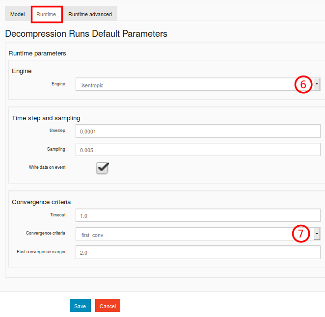
Fig. 9.8 Project Definition (continuation)

Note

three possible convergence criterion are available: “H”, “first_conv” and “timeout”. In the tutorials, the convergence criteria “first_conv” will be used which means that the run will end if one of the internal volume pressure reaches the external pressure before the time out specified (for more information on convergence criteria please refer to convergence criteria).

Once you saved, you will be redirected to your new project central page.

Step 6: launch your analysis¶

Click on the New Run button. You will be redirected to a form (Fig. 9.9).

By button “Browse” select your spreadsheet. All the other parameters have been defined as default parameters from the model.

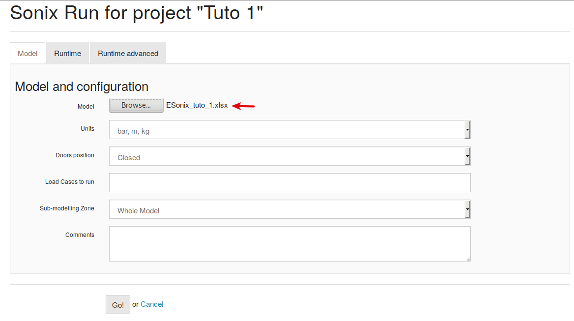
Fig. 9.9 New Run Form

Once you clicked on “Go!”, calculations are performed.

Check the results: the “results” page¶

The results can be easily accessed clicking in the Run Status, as per Fig. 9.10.

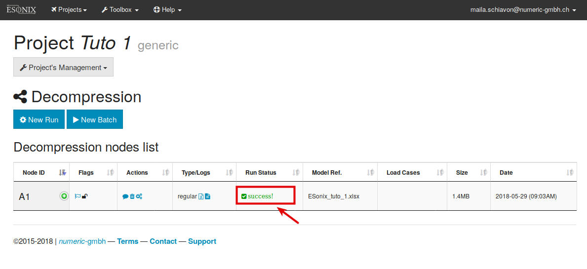
Fig. 9.10 Accessing results

“Downloads” Section¶

This section provides several spreadsheet as deliveries, such as Δp envelops, events chronologies, etc.

Curves plotting¶

You can plot different kind of values against time by following the appropriate link “dynamic plotter”. For example, let say you wish to check the evolution of Pressure and delta-pressure between volumes 1 and 2 (Fig. 9.11)

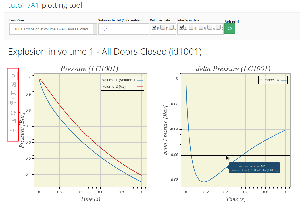
Fig. 9.11 Plotting variables over time using the dynamic plotter

Plots are dynamic: you can move the mouse over the curves to get data. But you can also zoom on the figures by scrolling the mid-button.

Conclusion¶

You learnt through out this tutorial the basics to prepare, run and check a very basic model.

download ESonix_tuto_1.xlsx

9.2. Tutorial #2¶

We will start from the model created for the Tutorial #1.

You can download this model from here:

download ESonix_tuto_1.xlsx

This model idealizes its two internal vents as passive vents, i.e venting area is constant over time.

To go one step forward, we will now learn how to idealise active vents such as decompression panels, and how to create multi-load case analysis.

Node A1: Same model, 3 load cases¶

To get some more fun, we will first introduce a multi-load case analysis by adding two additional load cases to the first model.

Rename the previous model to “ESonix_tuto_2a.xlsx”. Edit it to reflect the following proposal:

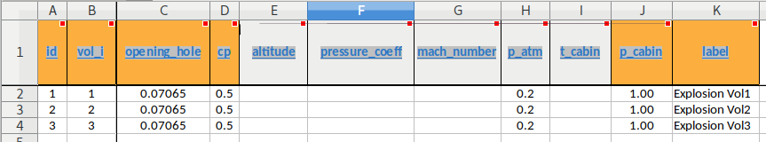
Fig. 9.12 load cases Definition

We basically created three load-cases: each of it simulating an opening in a different volume.

Create a new project “tuto 2” on Esonix. To have a reference to compare our next runs, let’s run this model with the same parameters as the ones used in “tuto 1”.

Warning

Watch the units and engine! When defining the new run, take care to specify the correct units and engine! The correct ones for this tutorial are “bar, m, kg” and “isentropic”.

Node A1: explore some of the Esonix pages¶

The node results page¶

You will be redirected to the results page. Find the Overview section, and unfold the panel “Main Deck to Main Deck”.

Two graphs are shown there:

a heatmap showing the maximum absolute value for each load case and each defined interface.
a bar plot summarising the max values for both directions for each interface.

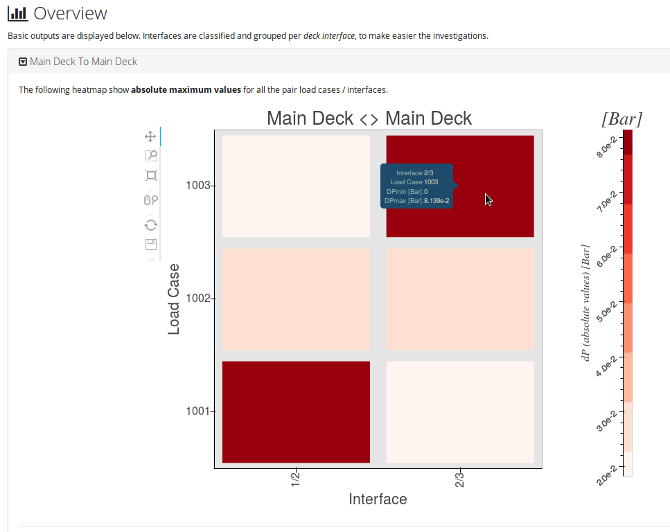
Fig. 9.13 Main deck to main deck heatmap

Fig. 9.14 Main deck to main deck histogram

Warning

Interface definitions and sign of \(\Delta_P\)

From the last figure, we can check that the maximum \(\Delta_P\) for interface “1/2” is \(+0.081\ bar\) for pressure acting from 2 to 1, and \(+0.02\ bar\) for pressure acting from 1 to 2.

The project page¶

From the previous run results page, you can go back to the project by clicking on the project name, at the top of the page.

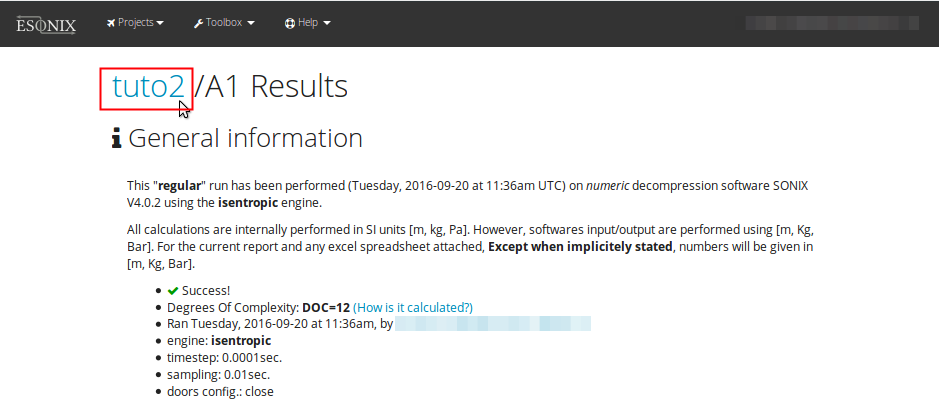
Fig. 9.15 Back to the project main page

From there, you can see that a “Decompression nodes list” was created. Here will be tabulated all the runs you will perform for a given project.

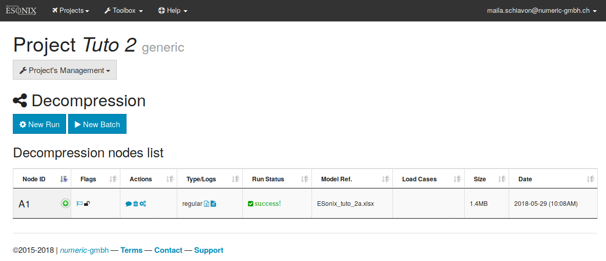
Fig. 9.16 Project nodes list

Let’s go quickly trough the line to explain the symbols. Some of them will show some useful tooltips when hovered.

Fig. 9.17 Project nodes list Icons

The columns shown in (Fig. 9.17) are:

Node ID (“A1”). This node ID is the identification number for this run .The next run will be called “A2”, etc.
Foldable access to see detailed information about Node “A1”.
Set the node as official.
Lock: An analysis cannot be deleted if the lock is “on”.
Comments symbol: By clicking on it, you can append some comments to your run. This helps to keep track of important information.
Trash: Click on it to delete the files.
Postprocess: Click on it to redo post-processing. Usually not useful except after an update of the software to gain access to an eventual new feature.
Type of analysis (here is “regular”). Different kind of analyses can be run. The simplest one is identified as “regular”. You can have as well “combinations” and comparisons” analysis.
Shortcut to Model excel spreadsheet referring to Node “A1”.
Shortcut to Analysis logs.
Access to the results main page. Green if the run was fine, red if something bad happened and no results are available.
Model reference used by the Node.
Load Cases covered by the Node. Empty field when all load cases defined in the Node were analysed.
Degree of Complexity (doc).
Run date and time (server time – UTC+1).

Node A2: Decompression panel¶

In place of the current passive vent between volumes 2 and 3, we now have to simulate a decompression panel with the following characteristics:

Full frame Area = \(0.07065\ m^2\) (as before)
Opening time = \(0.2\ sec.\) to get the full area.
Pressure release = \(0.15\ bar\)
The panel is supposed to open in both directions.

Copy your “ESonix_tuto_2a.xlsx” to “ESonix_tuto_2b.xlsx”, and edit it to reflect this:

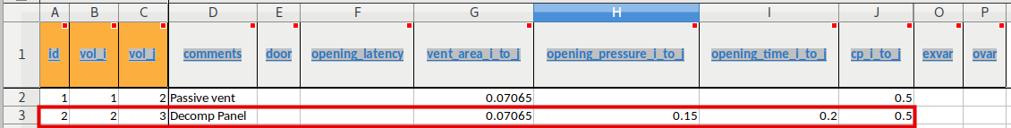
Fig. 9.18 Defining connections for decompression panel

Since the panel is supposed to have the same characteristics for both directions (from volume 2 to 3 and from volume 3 to 2), no need to edit the j_to_i columns: they will be automatically copied from the i_to_j columns.

Create a New Run and run the model “ESonix_tuto_2b.xlsx” to generate the Node A2.

From the A2 results page, go to the “overview” section as before, and compare the results we have now compared to A1.

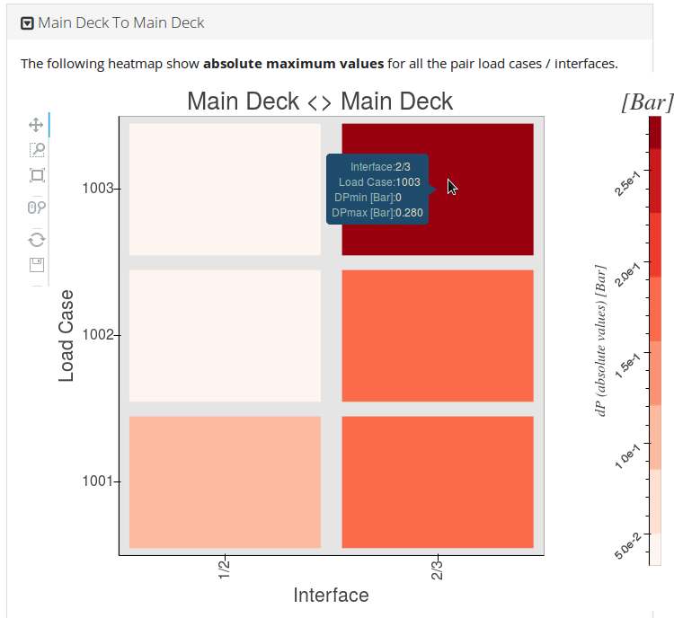
Fig. 9.19 A2 main deck to main deck Heatmap

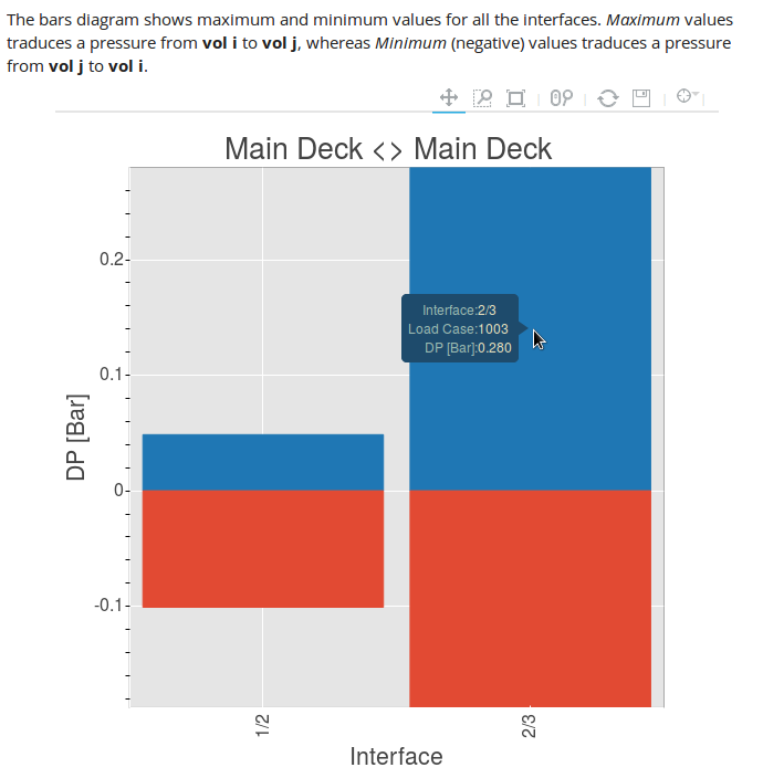
Fig. 9.20 A2 main deck to main deck histogram

Whereas results were “symmetric” for node A1, the decompression panel we introduced decreased maximum pressure that interface 1/2 was reacting, and increased the maximum pressure the interface 2/3 reacts, whatever the direction we check.

We can go one step further and investigate what happens with interface 2/3: click on the “Dynamic plotter”, as shown in Fig. 9.21.

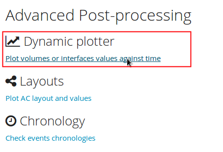
Fig. 9.21 dynamic plotter hyperlink

We will plot \(\Delta_P\) and \(Area\) for interfaces “1/2” and “2/3” for load case 1003, as shown in Fig. 9.22.

Select:

Load Case: 1003
Volumes to plot: enter “1,2,2,3”, to be understood as 1/2, 2/3
Values to plot: check “Δp” and “A” (delta pressure and Area)

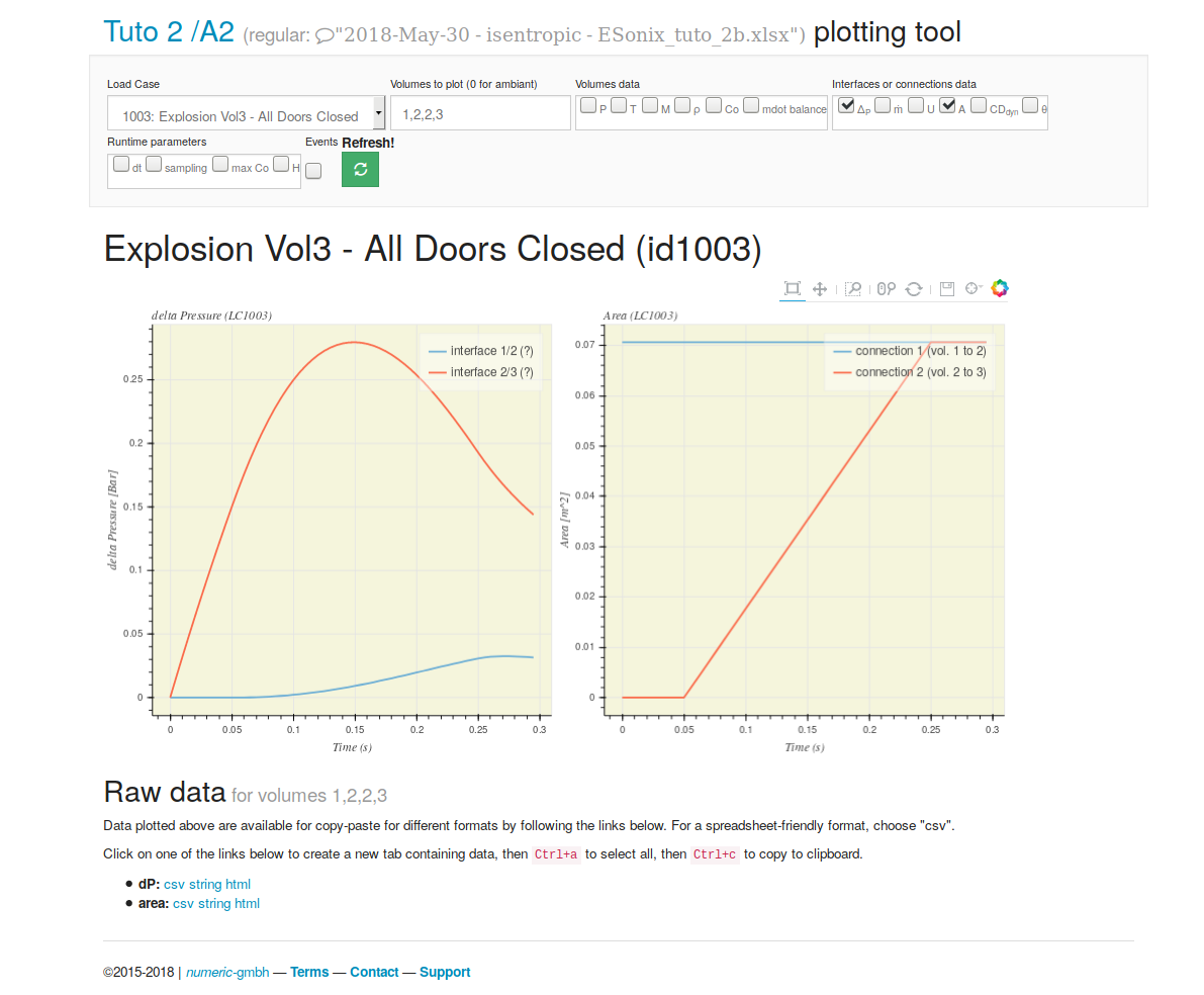
Fig. 9.22 Curves for interfaces 1/2 and 2/3

From the Area curves (on the right), it is clear that connection ID2 starts to open around 0.05 second, which is the time where \(\Delta_{P\ 2/3}\) reaches the released pressure (\(0.15\ bar\)).

DeltaP values from XLS results files¶

You can double check this opening behaviour from the “download section”.

Go back to the A2 results page (Fig. 9.23)and download the Δp spreadsheet (Fig. 9.24).

Fig. 9.23 Back to node’s main page!

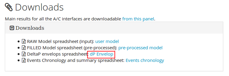
Fig. 9.24 Download node A2’s Δp spreadsheet

The first tab from the XLS files is titled Interfaces envelop and shows the envelop by interface (Fig. 9.25).

Fig. 9.25 per interface Δp envelop tab

The max \(\Delta_P\) for interface 2/3 is thus \(0.28\ bar\) (column absmax_v), occurring at \(0.1501\ sec\) (column absmax_t) and for load case 1003 (column lcid_absmax)

The second tab from the XLS files is titled LoadCase envelop and shows the envelop by load case. We highlighted in Fig. 9.26 the envelops for load case 1003.

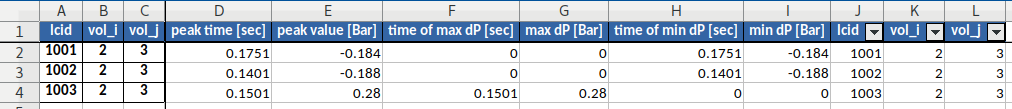
Fig. 9.26 per load-case Δp envelop tab

As expected, the max value highlighted from the by-load case envelop is the same as the highest value from the by-interface envelop.

Another interesting check is that the interface 2/3 is always critical, whatever the load case.

Chronology from XLS results files¶

Downloading the “Events chronology” spreadsheet provides summary to events occurring during the decompression.

From Fig. 9.27, we can double-check that the connection we defined with ID 2 (between volumes 2 and 3) is opening for a DeltaP=0.15 bars, and its opening is running for 0.2 seconds, from t=0.050 seconds to t=0.25 seconds.

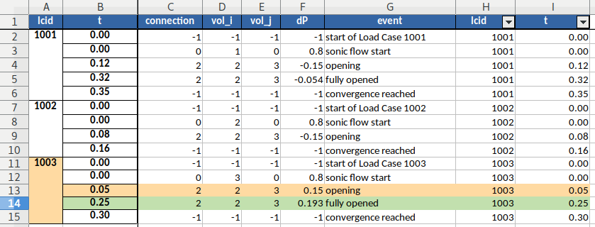
Fig. 9.27 Chronologies for all the load cases. Coloured lines highlight the opening of connection ID2 (0.2 seconds).

Downloads¶

You can download the models used through out this tutorial here under:

node A1: download ESonix_tuto_2a.xlsx
node A2: download ESonix_tuto_2b.xlsx

9.3. Tutorial #3¶

The Tutorial #1 refers to ESonix basics, Tutorial #2 explores basic decompression features definition, we will now explore how to define a door.

What is a “door” for ESonix?¶

Actually, a “door” as seen from ESonix, is not a decompression feature.

For ESonix, the concept of “door” is useful to define a fully static vent that is either opened or closed, depending on the configuration ran.

From the ESonix Excel template file, you can tag a connection as “door” by filling the “door” column. If a connection is identified as a door by ESonix, the corresponding path area will be cleaned when ESonix runs an “Opened door configuration” run. Obviously, the path will be closed for a “Closed door configuration”.

That being said, a door can act:

as a full decompression feature (e.g.: swivel doors) if the “vent_area_*” has the same value as the “door” column value.
as a nested decompression feature (e.g.: decompression panel) if the “vent_area_*” is lower than the “door” column value.

A connection tagged as “door” with a “vent_area_*” value equal to 0 will always be closed during a “Closed door configuration”.

Some more info can be found in the dedicated section doors, and in some useful common examples, like Simple decompressing door.

Defining a swivel door that doesn’t decompress: A1¶

To save some time, we will start from the second model created during the Tutorial #2. You can download ESonix_tuto_2a.xlsx, and save it as “Esonix_tuto_3a.xlsx”.

In place of the current decompression feature between volumes 2 and 3, we now have to simulate a swivel door that does not decompress. All the other parameters remain the same:

Full frame Area = \(0.07065\ m^2\) (a hobbit door, as before)
Opening time = No need as the door does not decompress.
Pressure release = No need.
Discharge coefficient CP = 0.5

Fig. 9.28 shows the modified model spreadsheet.

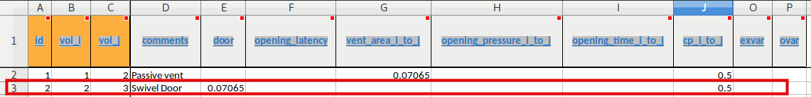
Fig. 9.28 Connection #2 is a simple non-decompressing door.

Connection ID2 is defined as “door” by filling the door column. Since the door is not supposed to decompress, vent_area_i_to_j and vent_area_j_to_i are set to zero (or let blank).

Run the simulation, for both opened and closed configurations¶

Create a new project called “tuto3”, preset it with appropriate units, and select “Opened AND Closed” configuration. Do not forget to select appropriate units “bar, m, kg”, engine “isentropic” and set the convergence criteria to “first_conv”.

Then run the first node with the modified spreadsheet. Since you selected “Opened AND Closed” and defined three load cases (one explosion per compartment), ESonix will therefore run six load cases:

All doors closed, explosion in volumes 1: Load Case 1001
All doors closed, explosion in volumes 2: Load Case 1002
All doors closed, explosion in volumes 3: Load Case 1003
All doors opened, explosion in volumes 1: Load Case 2001
All doors opened, explosion in volumes 2: Load Case 2002
All doors opened, explosion in volumes 3: Load Case 2003

Note

Load Cases numbering

ESonix will translate the Load Cases IDs defined from your model in two series:

1000 + Load Case ID for an “All Doors Closed” configuration
2000 + Load Case ID for an “All Doors Opened” configuration

Check the node A1’s results¶

What can we expect?¶

For the “Doors Opened” configurations (load cases 2001 to 2003), the problem is symmetric, and we expect \(\Delta_P\) for interface 1/2 and 3/2 need to be the same, as all the air path are equal.

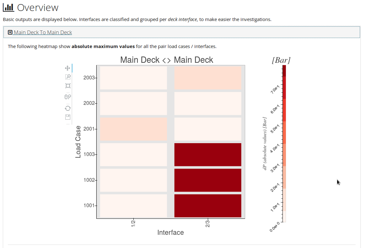
Fig. 9.29 Main deck to main deck A1 heatmap

For the “Doors Closed” configurations (load cases 1001 to 1003), the volume 3 will always be isolated from the rest of the cabin: the door will stay closed as no decompression feature is provided. Final Δp between volumes 2 and 3 should be equal to initial Δp between cabin and atmosphere (thus 0.8 bar).

This is the case for LC1003 only. For LCS 1001 and 1002 decompression time are longer than the 1 second assigned by default to the run (cf. advanced settings), and the air from volumes 1 and 2 has not fully exhausted to ambient.

Defining a decompressing swivel door: A2¶

We now want to change this door useless for decompression to a single-way decompressing swivel door. Let’s say we need a door opening at 0.15 bar, and reaching its full opening in 0.2 seconds (which is quite long).

In that purpose, we just need to specify an opening area equal to the door’s frame (thus 0.07065 m²), as the full door is opening.

Copy your initial file to “ESonix_tuto_3b.xlsx”, and change the “Connections” tab to match Fig. 9.30.

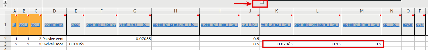
Fig. 9.30 Connection #2 is a swivel decompressing door.

Since we want the door to open from volume 3 to volume 2, we need to specify the values for the j_to_i columns. Discharge coefficients CP is valid for both ways, and specify it in the i_to_j columns is enough: it will be copied to the j_to_i values. It would have been ok though to specify it again.

Launch the run as before (“Opened and Closed”, “bar, m, kg” and “isentropic”), and check this new set of results (should be node A2).

Check the node A2’s results¶

What can we expect?¶

The most obvious result we expect is for an explosion in volume 3 and all doors closed: since the door is opening from 3 to 2, the door should never open, and maximum \(\Delta_{P\ 2,3}\) should be equal to initial \(\Delta_P\) between cabin and atmosphere (thus \(0.8\ bar\)).

We can easily check it from the heatmap Fig. 9.31.

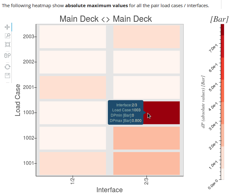
Fig. 9.31 Main deck to main deck A2 heatmap

We could also check it from the curves tool by plotting the venting area for interfaces 1,2 and 2,3 and for load case 1003 (Fig. 9.32).

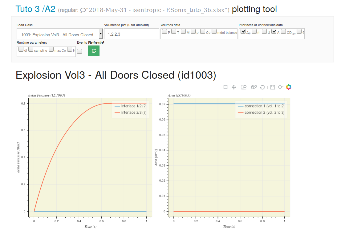
A2 dp and Area for interfaces 1/2 and 2/3 for load case 1003

Fig. 9.32 A2 Δp and Area for interfaces 1/2 and 2/3 for load case 1003

It is clear from the Fig. 9.32 that area for interface 2,3 remains 0, and that \(\Delta_{P\ 2,3}\) converges to \(0.8\ bar\).

If we plot the same data but for Load Case 1002 (explosion in volume 2 for an initial cabin configured with all doors closed, we can expect the door to open in the defined 2 seconds, and \(\Delta_{P\ 2,3}\) converges to \(0\ bar\). This is shown Fig. 9.33.

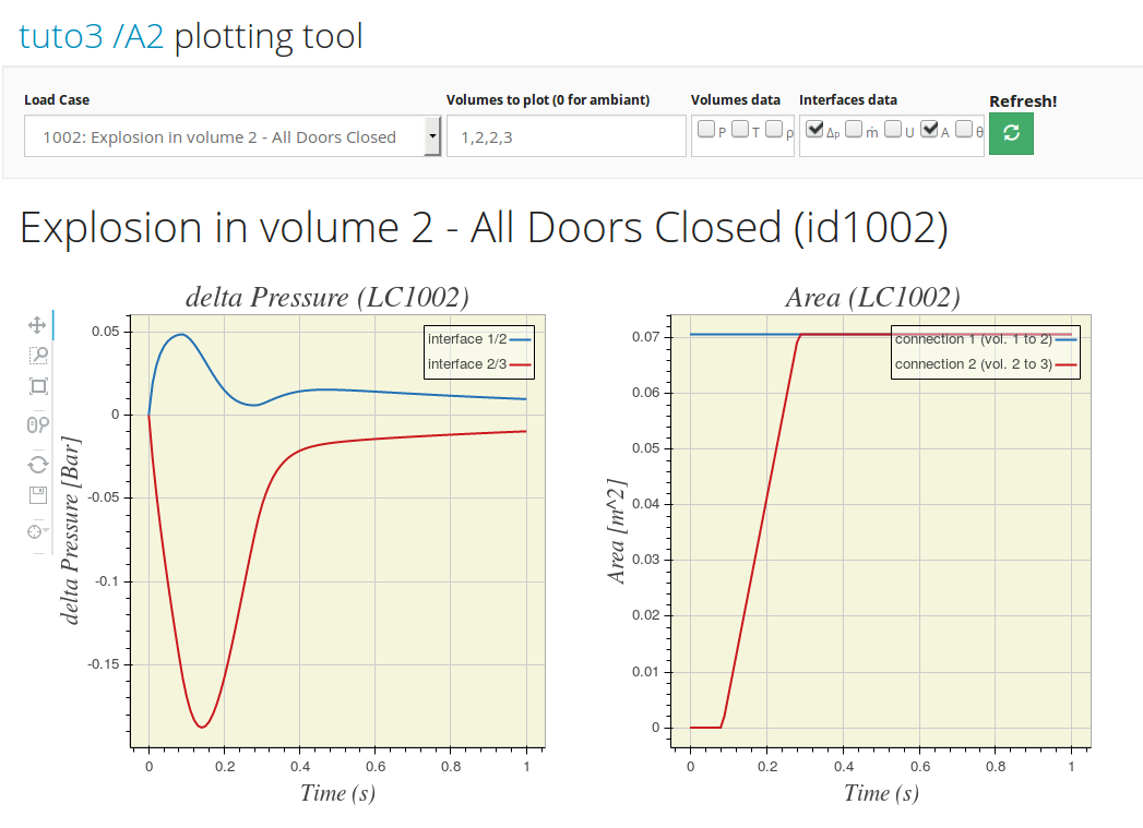
A2 dp and Area for interfaces 1/2 and 2/3 for load case 1002

Fig. 9.33 A2 Δp and Area for interfaces 1/2 and 2/3 for load case 1002

Defining a door hosting a decompression panel: A3¶

If the same swivel door as defined above would feature a decompression panel, assuming the decompression panel (let say a 0.03m²) opens in both directions, the door would have to be defined as (cf. Fig. 9.34)

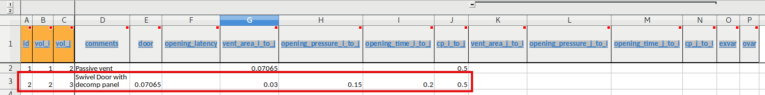
Fig. 9.34 Connection #2 is a swivel door hosting a nested decompression panel

The user is invited to modify the file “ESonix_tuto_3b.xlsx” as per Fig. 9.34, save it as “ESonix_tuto_3c.xlsx”, launch a New Run and check the results in comparison with previous results.

Defining a decompressing swivel door with dynamical attributes: A4¶

We defined in Defining a decompressing swivel door: A2 (node A2) a decompressing swivel door. To simulate the time the door will use to completely open, we set an opening time equal to 0.2 seconds.

Defining the opening time for all decompressing features can be heavy, and will necessarily be an approximation as opening time depends on real pressure acting on the item.

As of ESonix version 3, dynamical attributes may be added on already defined decompression items. Documentation tab “Dyn_Attributes” describes the way to do so: it mainly consists in adding a new tab to the basic model: dyn_attributes.

The easiest way is to download the “advanced template” as proposed from the “help” menu (Fig. 9.35).

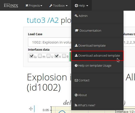
Fig. 9.35 Download the “advanced template” from the “help” menu

Copy the “Dyn_Attributes” tab to the spreadsheet used for node A2 (“ESonix_tuto_3b.xlsx”) and save it as “ESonix_tuto_3d.xlsx”. The node A2 was used to simulate swivel decompressing door.

Assuming the door will be a square panel with the same area as initial door, and a mass of 15kg, fill the Dyn_Attributes spreadsheet as shown in Fig. 9.36.

Fig. 9.36 Connection #2 is a swivel decompressing door with a dynamical behaviour.

The user is invited to launch a New Run and check the results in comparison with previous results.

Downloads¶

You can download the models used through out this tutorial here under:

9.4. Tutorial #4¶

This tutorial starts a new example from scratch. It is however recommended to practice with tutorials Tutorial #1, Tutorial #2 and Tutorial #3 before training with this one.

Presentation of the problem¶

This tutorial is based on [PC16], §5.4 “Four-Compartment aircraft”.

It will be studied an Aircraft made of three volumes at the main deck and one single cargo (Fig. 9.37). To characterise the influence of an occupied cargo, two models will be studied:

Cargo empty volume = 67m³ (model A)
Cargo occupied with a rate of 60% occupancy (therefore, cargo volume =67m³-60% = 26.8 m³ (model B)

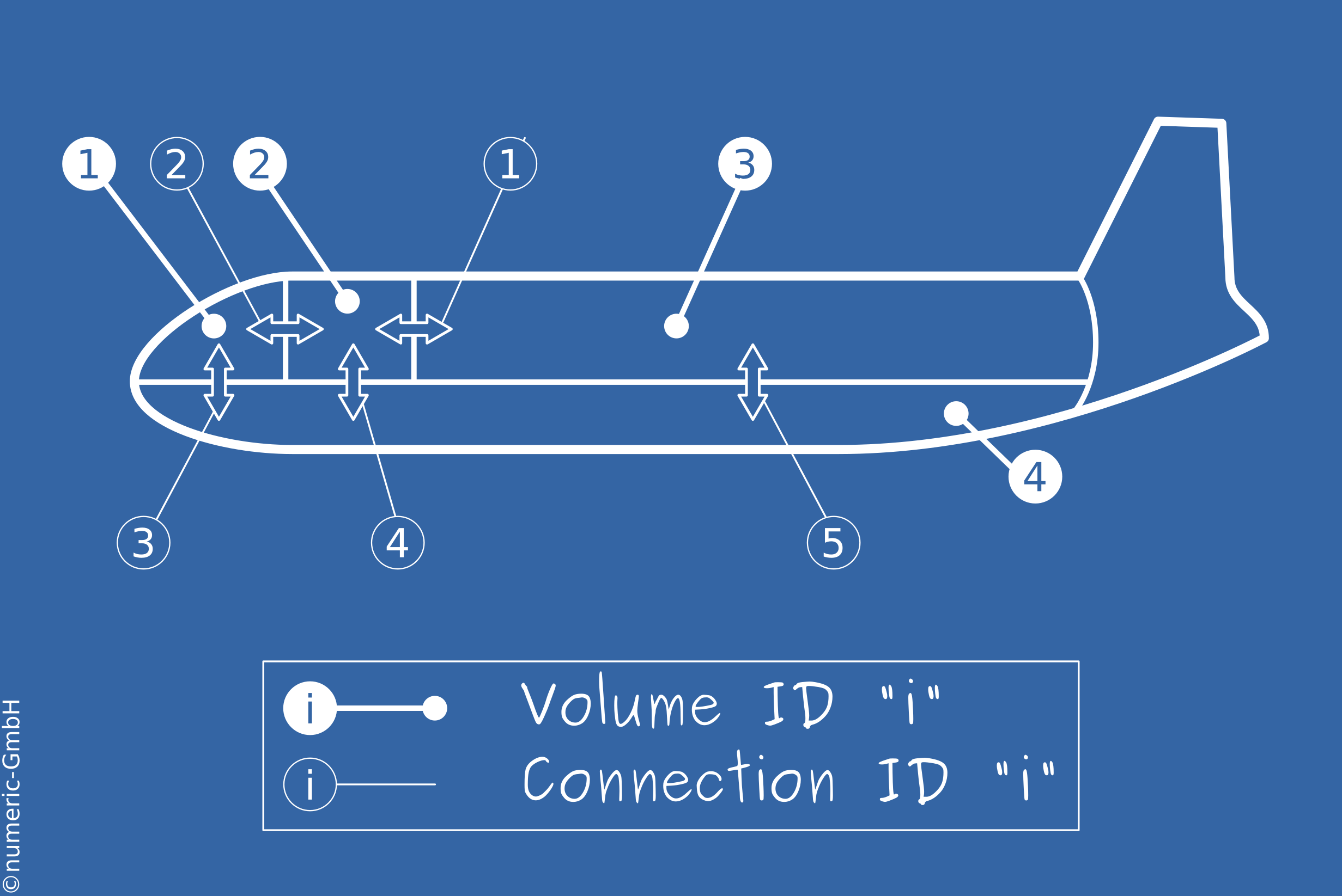
Fig. 9.37 Four volumes definition

Those two models will be ran to create two nodes A1 and A2. A sensitivity analysis will be performed on those two nodes to create node A3. This sensitivity analysis will be used to understand the influence of the cargo occupancy.

Once the critical configuration will be found using sensitivity analysis, we will create two models (A4 and A5) to be combined in a single set of results (node A6).

Lastly, a unified model will be created to show the basics of model unification (node A7).

Empty Cargo Volumes definition (model A)¶

The following values will be used:

Table 9.1 Four volumes Aircraft Volumes definitions (model A)¶
ID	label	volume
1	Cockpit	4m³
2	Entryway	3m³
3	Cabin	198m³
4	Cargo empty	67m³

Pressure cabin is given to 89.786 kPa (0.89786 bar), Temperature in the cabin is 23°C (296.15K)

Occupied Cargo Volumes definition (model B)¶

The volume of the cargo is reduced by 60%. New volume is therefore set to 26.8m³.

Table 9.2 Four volumes Aircraft Volumes definitions (model B)¶
ID	label	volume
1	Cockpit	4m³
2	Entryway	3m³
3	Cabin	198m³
4	Cargo occupied	26.8m³

Same cabin pressure and temperature as model A are used.

Connections definition (models A and B)¶

For Both models (model A and model B), compartments are connected as follows:

Table 9.3 Four volumes Aircraft Connections (models A and B)¶
ID	type	vol_i	vol_j	length	width	release pressure	Discharge Coeff.	Weight
1	passive	2	3	1.8 m	0.5 m	na	0.7	na
2	Vertical hinged blowout	1	2	0.447 m	0.447 m	0.06 bar	0.7	2.43 kg
3	translational blowout	1	4	0.3 m	0.3 m	0.04 bar	0.7	2.43 kg
4	translational blowout	2	4	0.3 m	0.3 m	0.04 bar	0.7	2.43 kg
5	translational blowout	3	4	0.3 m	0.3 m	0.04 bar	0.7	2.43 kg

Note

the blow out panel axis definition is important for dynamical opening behaviour and the setting parameters are specified in the user manual Dyn_Attributes/axis

Load Cases¶

For both models, the following settings are used:

Aircraft is flying at 9980 m. Authors provide ISA conditions Pa=26.5 kPa (0.265 bar) and Ta = -49.85°C (223.3 K).

Cabin Pressure will be kept equal to 89.786 kPa, and cabin internal temperature is 23° (296.15K).

Three openings will be simulated, one for each volumes with the exception of the cockpit, all equal to 0.6 m², with a discharge coefficient CD=0.8.

Runtime parameters¶

The following parameters will be used:

timestep: 5E-05 sec
sampling: 1E-03 sec
timeout: 1 sec
convergence criteria: first_conv

ESonix models (nodes A1 and A2)¶

Two models are now prepared: ESonix_tuto_4a.xlsx and ESonix_tuto_4b.xlsx describing the problem presented above.

Volumes and Connections¶

Volumes and connections are easy to define. You can refer to previous tutorials, or to documentation tab “Connections” and tab “Volumes”.

Note

in this tutorial the volume location deck ought to be specified in the Volumes tab (-1 for cargo volumes and 0 for main deck volumes)

Models are available (Downloads) to download for an easy check.

Dynamical attributes¶

The tab “Dyn_Attributes” defines the dynamical attributes as follows:

Fig. 9.38 Dynamical Attributes for models A and B

The hinged blowout panel between volumes 1 and 2 (connection #2) has a vertical rotation axis, therefore axis=0. No air drag is taken into account, hence cx=0. The flap can open in both directions, from where max_opening_i_to_j = max_opening_j_to_i=90°. To match as much as possible [PC16], we deactivate the following pressure (following_pressure=0) and set the opening_area_method to 1.

Note

for more information about Dynamical attributes please refer to the section 5.6 of the User Manual tab “Dyn_Attributes”

Load Cases¶

Load cases are defined as shown Fig. 9.39 (tab “LoadCases”):

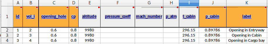
Fig. 9.39 Load Cases for models A and B

Note

the atmospheric pressure can be defined either directly in the column p_atm or via the flight altitude in the column altitude however they can’t be both defined at the same time for consistency purpose.

A3: Sensitivity analysis¶

Once “tuto4” project created (use “isentropic” engine, time step dt=0.00005 and sampling=0.001, all doors closed) run model A, then model B. The project page should look like Fig. 9.40.

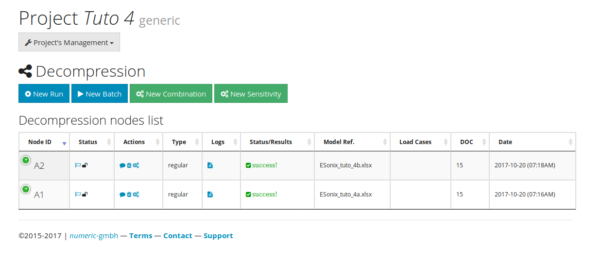
Fig. 9.40 Nodes A1 and A2 before combination

Click on “New Sensitivity” to create node A3. A form (Fig. 9.41) allows you to select reference node (here, select node A1), then all the nodes to be compared (here node A2 only). Then click on “Sensitivity” button to launch the analysis.

Fig. 9.41 Form to generate a sensitivity Analysis between nodes A1 and A2

Once the run is performed, you are redirected to the newly created A3 node.

The first look should be given to bar graphs and heatmaps available in the “Overview” section. As per regular nodes, overview panels are organised per deck interface (cf. Overview panels).

Cargo to Main Deck sensitivity¶

The sensitivity to the occupation of the cargo for the floor structure can be checked from the “Cargo to Main deck” data.

Contrary to heatmap from regular nodes, sensitivity heatmap shows standard deviation for each pair of load case and interface. The greatest the value, the greatest the difference.

The heatmap for main deck to cargo interfaces clearly show that having a cargo full or occupied mainly impact Load case 1003, and this for all the interfaces (cf. Fig. 9.42).

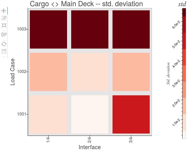
Cargo empty/occupied Sensitivity Heatmap

Fig. 9.42 Standard deviation for cargo empty or occupied –main deck to cargo interfaces–

Bars graphs will show Δp peaks values for each interface models have in common. If an interface would exist in a model, and not in one of the others, the interface would be omitted.

This graph is handy to check which one of the model is the most critical. Fig. 9.43 clearly shows that occupied cargo is critical for the main deck to cargo interfaces, therefore, for the floor structure.

The X axis is built with each interface of each node (“i/j/Node”): “1/4/A1”, “1/4/A2”, “2/4/A1”, “2/4/A2”, etc.

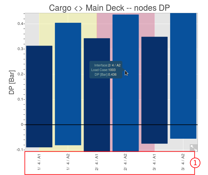
Fig. 9.43 Side by side peaksor cargo empty (A1) or occupied (A2) –main dack to cargo interfaces–

Moving the mouse over the bar graph pops up some tool tips providing some more info about the graph. From those tool tips, all the positive values (from volume x to volume 4, where x is one of {1, 2, 3}) traduce pressure from volume x to volume 4, therefore downward pressures. More over, all the positive values come from load case 1003 (explosion in the Cargo).

Plotting comparative graphs can be done using the dynamic plotter (cf. Fig. 9.44)

Dp for interface 1/4, loadcase 3 (Opening in Cargo)

Fig. 9.44 Δp for interface 1/4 and nodes A1 and A2, loadcase 3 (Opening in Cargo)

Another way to display detailed decompression information is to use the Layouts tool. If the location of all volumes are properly set up (Volumes deck, sta and rbl of the model) volume and connection info can be displayed on the Aircraft layout at any time of the decompression analysis.

Note

the Layouts tool is only available in Nodes created from regular analysis. In our case, the Layouts tool can be accessed in Node A1.

Fig. 9.45 Connection Δp, massflow and volume pressure at t=0.5s (LC1003)

In order to size the cabin, it is not convenient to switch between the two nodes, depending on the interface and the load case. This issue is addressed with Combination Analysis (cf. Combination Analysis for documentation).

A4: Combination¶

From Sensitivity Analysis conducted above, we determined that model A (cargo empty) is critical for explosion in the main deck and model B (cargo occupied), was critical for an explosion occurring in the cargo.

We will therefore modify models A and B as follows:

copy ESonix_tuto_4a.xlsx to ESonix_tuto_4c.xlsx, and delete load case #3 (Opening in Cargo).
copy ESonix_tuto_4b.xlsx to ESonix_tuto_4d.xlsx, and delete load case #1 and #2 (Openinges in main decks). For demonstration purposes, renumber the remaining load case ID as load case #1.

We now have two models: model A (ESonix_tuto_4c.xlsx) featuring explosion in the main decks with empty cargo, and model B (ESonix_tuto_4d.xlsx) featuring an explosion in the occupied cargo. Run those two models to create respectively Nodes A4 and A5.

Create now a combination analysis (button “New combination” from the project page). The New Combination form is quite similar to the sensitivity’s one. Select Nodes A4 and A5.

This will create the Node A6. Results page for a combination node is very similar to regular run results, although an additional “Combination Load Case Mapping” is provided.

Load case mapping is explained Combination Analysis. The load case mapping for Combination A6 is shown in the result page, panel “Combination Load Case Mapping” (item #2 from Fig. 9.46).

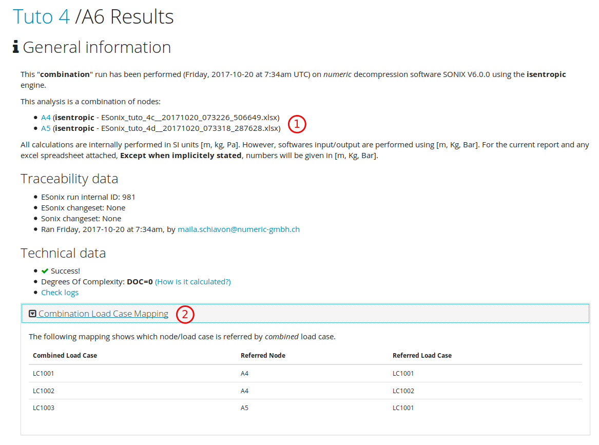
Fig. 9.46 Node A6: Combination results

The item #1 shows the Nodes that were combined. Several Nodes could be compared in a new Node. From the mapping table shown in item #2 from Fig. 9.46, we can see that node A6 has now three load cases (1001, 1002 and 1003), such as

A6/LC1001 is A4/LC1001 (explosion in entryway with empty cargo)
A6/LC1002 is A4/LC1002 (explosion in cabin with empty cargo)
A6/LC1003 is A5/LC1001 (explosion in cargo with occupied cargo)

Tip

Combination Analysis provides the same deliverable, graphs and tools as regular nodes!

With a Combination analysis, we can now check and build a decompression report based on a single set of results, with unique envelop, although two (or more) models are involved in the calculations.

Unified model¶

Combination Analysis is a great step towards a simple yet powerful Aircraft decompression analysis. However, in some cases like the one above, ESonix provides a simpler way to address the multiple models issue: the “Unified Model”.

A Unified Model is a classical ESonix model making use of one, several or all of the following parameters: deor, veor, ovar or exvar.

Those parameters let know to ESonix how to reinitialise the model for each load case.

For the current example, we will use the volume’s veor parameter. “veor” stands for “Volume Explosion Occupation Rate”. By setting Cargo’s veor parameter to 0.6, we let know to ESonix that this volume is reduced by 60% when this volume is the exploded volume.

Copy ESonix_tuto_4a.xlsx to ESonix_tuto_4e.xlsx, and set cargo’s volume definition veor parameter to 0.6 as shown Fig. 9.47, then run a regular analysis on it. This will create the last node of this tutorial: node A7

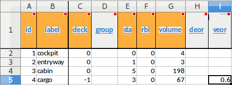
Fig. 9.47 A7 volumes definition

Results for the Unified Model A7 are the same as for the Combination Analysis A6.

Note

To go further

As an exercise, you could now perform a sensitivity Analysis for nodes A6 (Combined nodes) and A7 (unified model), and check that standard deviation heat maps show really low values.

Downloads¶

You can download the models used through out this tutorial here under:

Nodes used to build sensitivity analysis A3:

node A1 model: download ESonix_tuto_4a.xlsx
node A2 model: download ESonix_tuto_4b.xlsx

Nodes used to build combination analysis A6:

node A4 model: download ESonix_tuto_4c.xlsx
node A5 model: download ESonix_tuto_4d.xlsx

Unified model Node A7:

node A7 model: download ESonix_tuto_4e.xlsx

9.5. Tutorial #5¶

This tutorial explains the use of the Batch tool.

The Batch tool is a powerful tool that allows the users to run several Nodes (models), including combinations and sensitivities analysis, in parallel. The main goals of this tool is to save running time and keep an easier way to track all parameters considered in the analysis/investigations.

Presentation of the problem¶

The main goal of this Tutorial is to run in parallel all models, sensitivity and combination analysis from Tutorial #4, using the Batch tool.

The five models generated in the previous Tutorial #4 are available to download:

Note

For a better understanding of this tutorial and better understand of the Batch tool, the practice of the Tutorial #4 is recommended.

In order to run the Batch Tool the user needs: ESonix models (from Tutorial #4) and the Batch Command File. The Batch Command File will be written along this tutorial.

The Batch Tool is accessible by button New Batch, where, in the next step, the models and the Batch File need to be uploaded. See Fig. 9.48 and Fig. 9.49

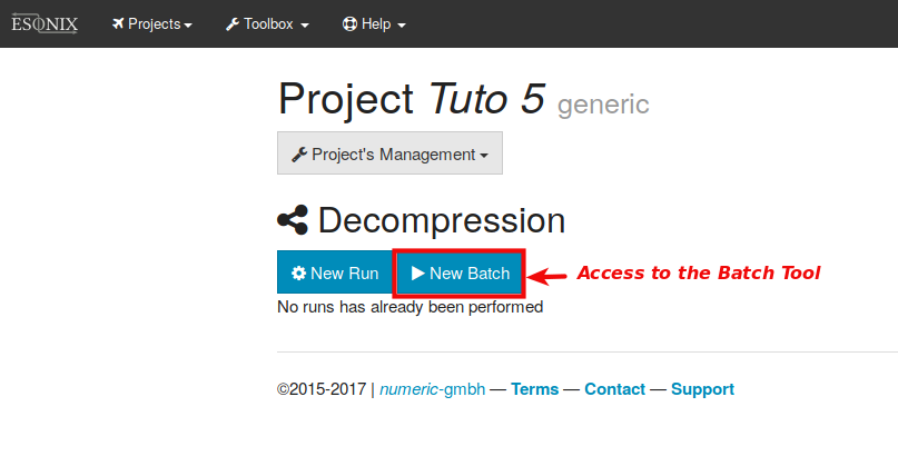
Fig. 9.48 Batch Analysis access button

.

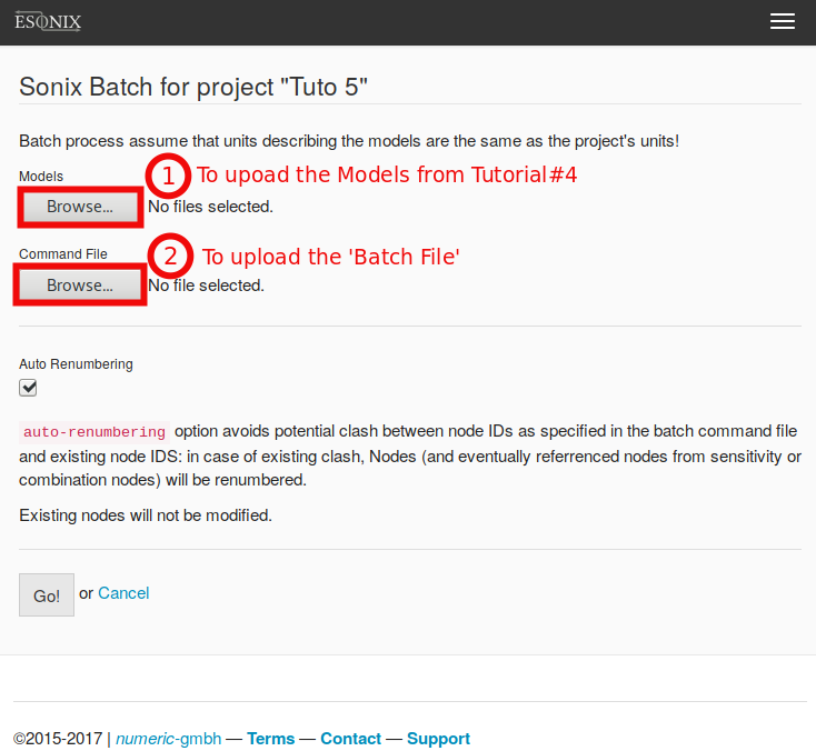
Fig. 9.49 Batch Analysis uploaded files access

Preparing the Command File¶

The Command File is a file where all information about the models and the analysis to be performed is stored. In addition, sensitivity and combination analysis can be also added in this file. All the standards analysis considered in the Batch File will be run in parallel. For the sensitivity and combination analysis their run will be triggered when the results of the dependent nodes will be available.

By the button Project Management two templates of Command File are available, see Fig. 9.50:

Batch Template: this template contains comments and general instructions to write a Command File. The use of this template is recommended for those starting with the Batch tool.
Minified Batch Template: this template omits comments and instructions to write a Command File. The use of this template is recommended for those feeling comfortable with the Batch Tool.

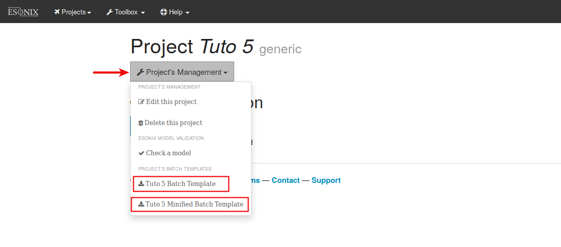
Fig. 9.50 Command File - template access

The Minified Batch Template will be used to write the Command File of this tutorial. The user should then dowload this template and follow the next steps. As shown by Fig. 9.51, three main sections may be considered in the Command File:

[regular analysis]: where the default parameters and Models are defined.
[combination analysis]: where combination analysis between Models may be defined. This section can be deleted in case no combination analysis is required.
[sensitivity analysis]: where sensitivity analysis between Models may be defined. This section can be deleted in case no sensitivity analysis is required.

Note

For additional information about ‘Batch Analysis’ and ‘Command File’, the user is invited to check the chapter Batch Analysis.

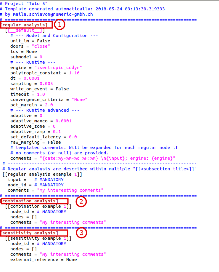
Fig. 9.51 Command File - Minified Template

—Step 1: Writing the [regular analysis] subsection—

The [regular analysis] subsection is divided in [[__default__]] subsection and models [regular analysis example 1, 2, 3, etc] subsection.

[[__default__]] subsection

The chapter Batch Analysis shows explanations for each parameter of the [[__default__]] subsection.

The [[__default__]] subsection for this Tutorial#5 is set based on the parameters of Tutorial #4 and can be written as:

[[__default__]}
    # --- Model and Configuration ---
    unit_im = False
    doors = "close"
    lcs = None
    submodel = 0
    # --- Runtime---
    engine = "isentropic"
    polytropic_constant = 1.16
    dt = 5E-05
    sampling = 0.001
    write_on_event = True
    timeout = 1.0
    convergence_criteria = "first_conv"
    pct_margin = 2.0
    # --- Runtime advanced ---
    adaptative = 0
    adaptative_maxcp = 0.0001
    adaptative_zone = 2
    adaptative_ramp = 0.1
    set_default_latency = 0.0
    raw_merging = False

[regular analysis example 1, 2, 3, etc] subsections

The chapter Batch Analysis shows explanations for each parameter of the [regular analysis example 1, 2, 3, etc] subsection.

Note

the value of the analysis parameters defined in the subsection [[__default__]]] can be overwritten with specific analysis values defined in the [regular analysis example 1, 2, 3, etc] subsection.

[[regular analysis 1, 2, 4, 5, 7]] of this tutorial are equivalent to Nodes from Tutorial #4. They are defined as:

[[A1]]
    input= "Esonix_tuto_4a.xlsx"
    node_id= 1
    comments= "Cargo Empty"

[[A2]]
    input= "Esonix_tuto_4b.xlsx"
    node_id= 2
    comments= "Cargo Occupied"

[[A4]]
    input= "Esonix_tuto_4c.xlsx"
    node_id= 4
    comments= "Cargo  Empty; LC1 and 2"

[[A5]]
    input= "Esonix_tuto_4d.xlsx"
    node_id= 5
    comments= "Cargo  Occupied; LC3->LC1"

[[A7]]
    input= "Esonix_tuto_4e.xlsx"
    node_id= 7
    comments= "Unified"

Warning

the file name is case sensitive and should be specified exactly as it appears in your file explorer.

—Step 2: Writing the [combination analysis] subsection—

In the chapter Batch Analysis subsection [combination analysis] explanations for each parameter can be found.

In the Tutorial #4, the Node A6 is a combination of Nodes A4 and A5. In the Command File this new Node A6 can be written as:

[combination analysis]

    [[combination A4 and A5]]
        node_id = 6
        nodes = [4, 5]
        comments = "Combination of A4 and A5"

—Step 3: Writing the [sensitivity analysis] subsection—

In the chapter Batch Analysis subsection `[sensitivity analysis] explanations for each parameter can be found.

In Tutorial #4 there are two sensitivity analysis. In the Command File these new Nodes can be written as:

[sensitivity analysis]

    [[sensitivity of A1 and A2]]
        node_id = 3
        nodes = [1, 2]
        comments = "sensitivity of A1 and A2"


    [[sensitivity of A6 and A7]]
        node_id = 8
        nodes = [6, 7]
        comments = "sensitivity of A6 and A7"

The Batch File of this Tutorial #5 can be downloaded here (download ESonix_tuto_5_batch.ini)

Running Nodes with the Batch Tool¶

To run the Batch Tool, we need to access it as shown by Fig. 9.48 and Fig. 9.49. The five models from Tutorial#4 (Downloads) can be then uploaded and the Batch File as well. The Models can now start to run in parallel.

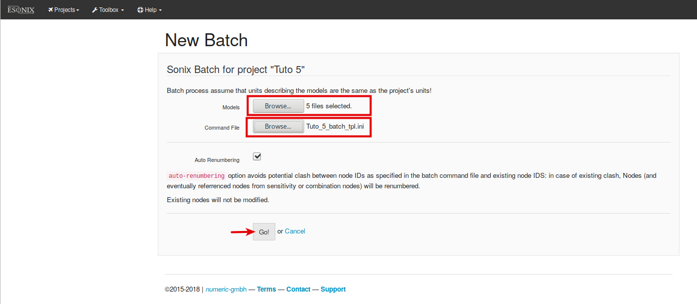
Fig. 9.52 Batch Tool - Files uploaded

The Fig. 9.53 shown as example all Models uploaded running in parallel.

The column 1 (Node ID) shows the Node ID corresponding to those previously defined in the Command File.
The column 2 (Type/Logs) describes the type of analysis. As defined by the Command File, there are two sensitivity analysis (Nodes #3 and #8), one combination analysis (Node #6) and five regular analysis (Nodes #1, #2, #4, #5, #7).
The column 3 (Run Status) informs about the run progress. In this example, the analysis of Node #1 to Node #7 are finished, while the sensitivity analysis of Node #8 is at 62.5% of progress.
The column 4 (Model Ref.) informs the Models reference in case of sensitivity or combination analysis OR the referred Excel file (Model).

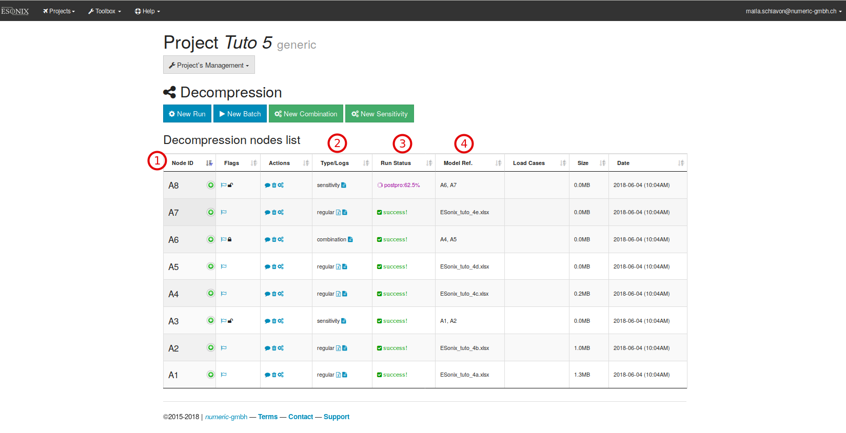
Fig. 9.53 Batch Tool - Example of models run in parallel

Conclusion¶

In this Tutorial#5 the same analysis performed in the Tutorial #4 were done through the Batch Tool and both tutorials present the same results (the user is invited to compare them as exercise).

The Batch Tool (see Batch Analysis) allows several runs in parallel saving time. In addition all information and parameters used in the several models are gathered in a single file, the Command File.

Downloads¶

You can download the models used through out this tutorial here under:

Batch command file: download ESonix_tuto_5_batch.ini

9.6. Tutorial #6¶

This tutorial aims to explain and to demonstrate the use of the Tweaks facility.

The Tweaks facility is accessible via an Excel sheet named Tweaks available in the Advanced Template, see Fig. 9.54.

The Tweaks facilities allows the user to modify (tweak) pre-defined parameters as: volume, cp, vent area, opening pressure, etc …, during the running time in order to dynamically modify the initial model to adjust it for specific load case configuration.

Problem 1 - Starting with Tweaks facilities¶

In the Problem 1 the last model of Tutorial #4 (ESonix_tuto_4e.slsx - Unified model) will be the reference model. The purpose of this exercise will be to reduce the cargo bay volume just for the explosion in cargo load case.

To be able to run a single model using the Tweaks facility, the Tweaks sheet need to be prepared with information of model ESonix_tuto_4e.xlsx.

Note

For a better understanding of this tutorial and comprehension of the Tweaks facility, the practice of the Tutorial #4 is recommended.

Quickly remembering the Tutorial #4:

The Tutorial #4 considers a four volume model, including Cargo Volume as shown in the Fig. 9.37.

The models consider three Load Cases: explosion in each volume with exception of the Cockpit.

In the model ESonix_tuto_4e.xlsx, the Cargo Volume was considered Empty (Cargo empty volume 67m³) for all main deck explosions and the Cargo Volume was considered Occupied (Cargo volume reduced by 60%: 67m³-60% = 26.8 m³) for an explosion in the cargo bay thanks to the use of VEOR parameter. In this tutorial, the VEOR parameter will be removed and replaced by a more generic “TWEAK parameter”.

Filling the Tweaks Excel sheet¶

The Tweaks tab can be filled as per following steps:

1st Step: Download the Advanced Template to have access to the Tweaks facility. The Advanced Template can be accessed by Help section of ESonix, see Fig. 9.54 .

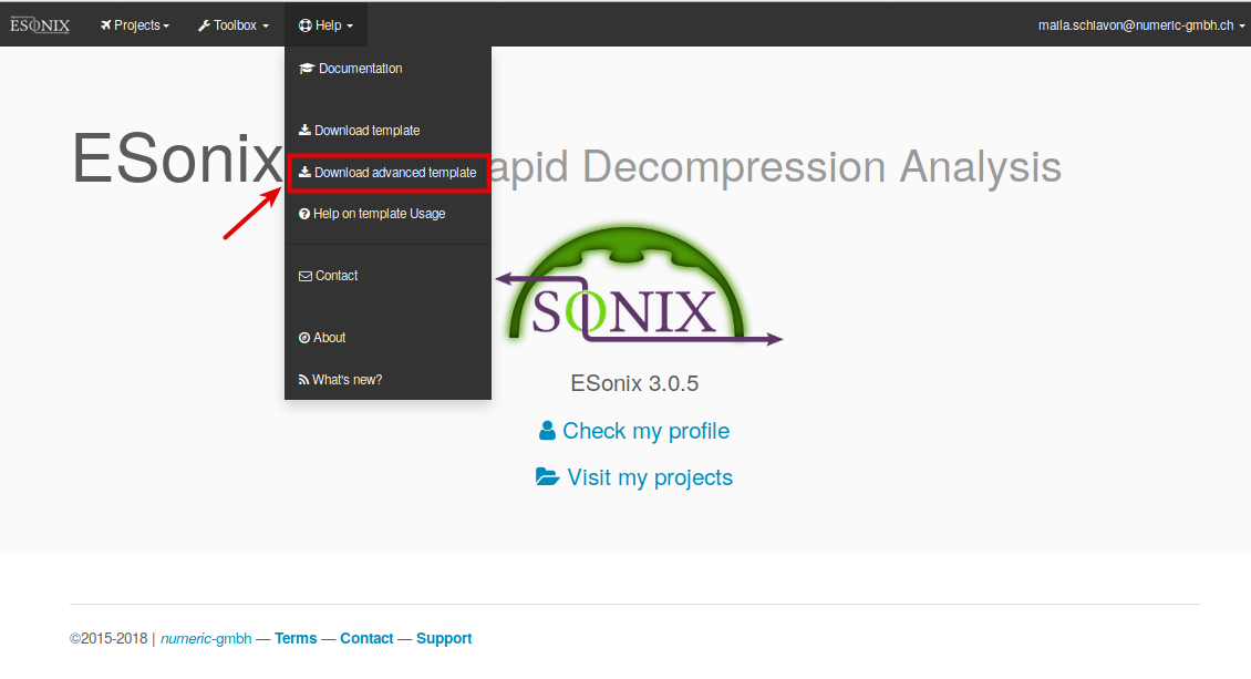
Fig. 9.54 Advanced Template - Download

2nd step: Download the last models from Tutorial #4:

download ESonix_tuto_4e.xlsx

3rd step: Make a copy of model ESonix_tuto_4e.xlsx and rename it as ESonix_tuto_6a.xlsx.

4th step: Delete the “VEOR parameter” in the Volume sheet

5th step: Add to this model ESonix_tuto_6a.xlsx the Tweaks sheet from the previously downloaded Advanced Template.

6th step: Add the TWEAK parameter to reduce the Cargo volume only for the explosion in Cargo volume.

The Tweaks Excel sheet of the model ESonix_tuto_6a.xlsx will be filled with value of Occupied Cargo. The columns 1 to 6 highlighted in the Fig. 9.55 are explained here after:

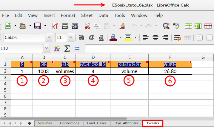
Fig. 9.55 Model ESonix_tuto_6a - Filled Tweaks Excel sheet

id: this column defines an ID for the Tweak parameter itself .
lcid: this column identifies the load case id for which the “tweaked parameter(s)” will be activated

To reproduce the model ESonix_tuto_4e.xlsx, only load case id 1003 will be here listed, as shown in Fig. 9.55.

Warning

load case defined here is load case id 1003 (load case id 3 with closed door configuration) and not load case id 3 because the TWEAK parameter could be applied independently to load case 1003: closed door configuration or load case 2003: open door configuration

tab: this column identifies the reference tab of the “tweaked parameter”.

To reproduce the model ESonix_tuto_4e.xlsx, the cargo volume need to be decreased. So, the Volumes tab is the one to be considered in our example, see Fig. 9.55.
tweaked_id: this column identifies within the tab selected, the corresponding id of the “tweaked parameter”.

To reproduce the model ESonix_tuto_4e.xlsx, the cargo volume id#4 of Volumes tab is the “tweaked parameter”.
parameter: this column defines the specific parameter to be modified. The parameter should refer to the column header.

To reproduce the model ESonix_tuto_4b.xlsx, the column volume of Volumes tab corresponding to the “tweaked parameter”.
value: this column defines the new value that should be considered by the “Tweaks facility”.

To reproduce the model ESonix_tuto_4e.xlsx, the Cargo volume need to be reduced by 60%. The Occupied Cargo Volume is then 28.6m³ for ony the Cargo load case.

7th step: Save the model ESonix_tuto6a.xlsx after modifications.

Running the model with the Tweaks Facility¶

There is no difference running a standard model or a model modified through Tweaks facilities.

Create a New Project and name it Tuto 6 (use “isentropic” engine, time step dt=5E-5, sampling=0.001, all doors closed, as per Tutorial #4 and convergence criteria=”first_conv”).

Upload and run model ESonix_tuto6a.xlsx. The project page should look like Fig. 9.56.

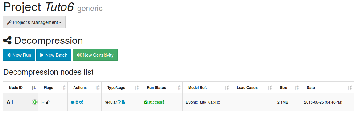
Fig. 9.56 Nodes A1 of Tutorial #6

The results from this analysis (ESonix_tuto6a.xlsx, Cargo bay volume occupancy modified through Tweaks facilities) should be compared with the results from the node A7 (ESonix_tuto4e.xlsx, Unified model, Cargo bay volume occupancy modified with VEOR parameter) of Tutorial #4. Unfortunately as those two sets of results belong to different projects they can’t be directly compared with the use of Sensitivity Analysis. However there is a possibility to perform this comparison automatically with ESonix. In order to achieve this comparison, the following Steps should be followed:

1st Step: In project Tuto4, Node A7, the dP Envelop should be downloaded.

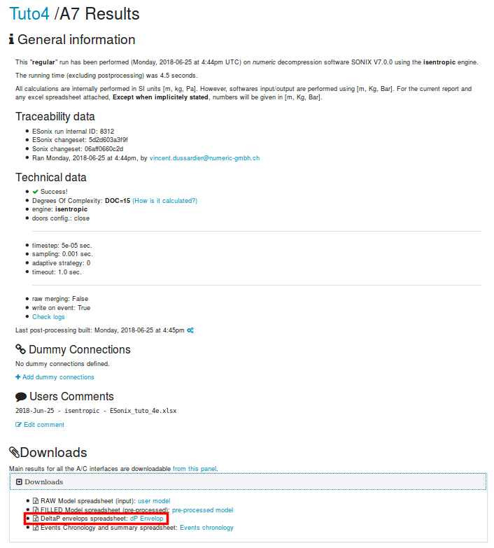
Fig. 9.57 Download results of Tutorial #4

2nd Step: In project Tuto6, a sensitivity analysis can be launch selecting the results of Node1 as the Reference node and the results stored in the downloaded EXCEL spreadsheet from Tuto04 Node A7 as the compared one.

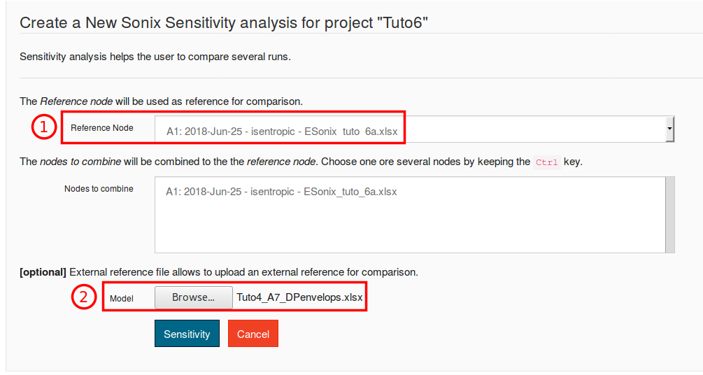
Fig. 9.58 Sensitivity analysis with external reference file

Hint

if the button “New Sensitivity” doesn’t appear after the run of node A1 is finish the web page should be refreshed in the hosting browser (usually F5 command).

As expected, the Sensitivity analysis between results from Node A7 of Tutorial#4 and results from Node A1 of Tutorial#6 show very low Standard Deviation (less than 1E-4) indicating that results are almost identical.

Note

As presented in this example the “TWEAK” parameter offers a different way to modified the cargo volume compared to the VEOR (Volume Explosion Occupancy Rate) parameter presented in Tutorial#4

Note

In the Problem 1 only one parameter was tweaked (the cargo volume); however it is important to highlight that any pre-defined parameter can be tweaked. In addition more than one parameter can also be tweaked in the same model, or one parameter can be tweaked with different values in different load cases. The Problem 2 shows additional possibilities of the Tweaks facilities:

Problem 2 - Going further with Tweaks facilities¶

To go further with the Tweaks facilities, the user is invited to save the model ESonix_tuto6a.xlsx as ESonix_tuto6b.xlsx. With this “new model”, the following steps should to be considered:

Step 1: A Cockpit Load Case will be added in the Load_Cases sheet. In order to match Load Case ID and exploded volume ID vol_i the existing load cases will be renumbered. The new load case will simulate a windshield breach with an opening hole of 0.4m² at the same altitude and cabin pressure/temperature as the other load cases.

Tweaks Excel Sheet - Additional modification

Fig. 9.59 Load_Cases Excel Sheet - Additional load case

Hint

it’s always a good idea to set the load case ID equal to the volume ID when possible as it will make the reading of decompression results handy Load case 1004 means explosion in the volume 4 with door initially closed

Step 2: Update the load case id of the first TWEAK parameter as the Cargo load case is now lcid 1004

Step 3: Save and run this model to generate a reference to evaluate the influence of the additional TWEAKS parameters on the connections

Step 4: Make a copy of the model ESonix_tuto6b.xlsx by saving it as ESonix_tuto6c.xlsx. This model will be now be modified with additional TWEAKS parameters (Step5 to 7)

Step 5: Increase the vent area between all volumes connected to the Cargo by 10% for load case 4 (LC4: explosion on cargo).

Warning

the TWEAKS parameters should be applied directly on the width and height of the decompression panels in the Dyn_Attributes Tab as those values are used to compute the dynamical opening area. (A 10% increase on the area means a \(\sqrt(1.1)=4.88\) % increase in the panel width and height)

Step 6: Increase the Opening Pressure between Vol1 (Cockpit) and Vol2 (Entryway) to 0.07 bar for Load Cases #2 and #3 - Only in this direction: Vol1 -> Vol2

Step 7: Decrease the Opening Pressure between Vol2 (Entryway) and Vol1 (Cockpit) to 0.04 bar for Load Cases #1 - Only in this Direction: Vol2 -> Vol1

The Fig. 9.60 shows Tweaks Excel Sheet with the modifications proposed.

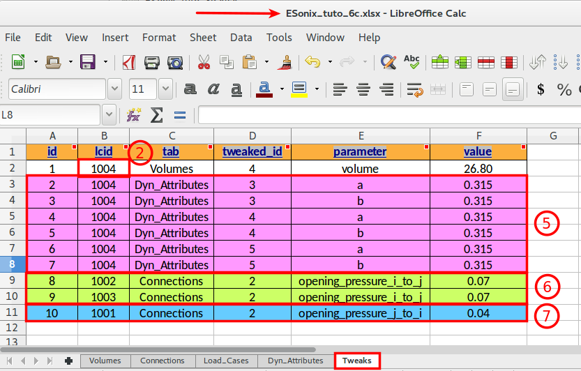
Fig. 9.60 Tweaks Excel Sheet - Additional modification

The Fig. 9.61 highlights the modifications considered in problem 2.

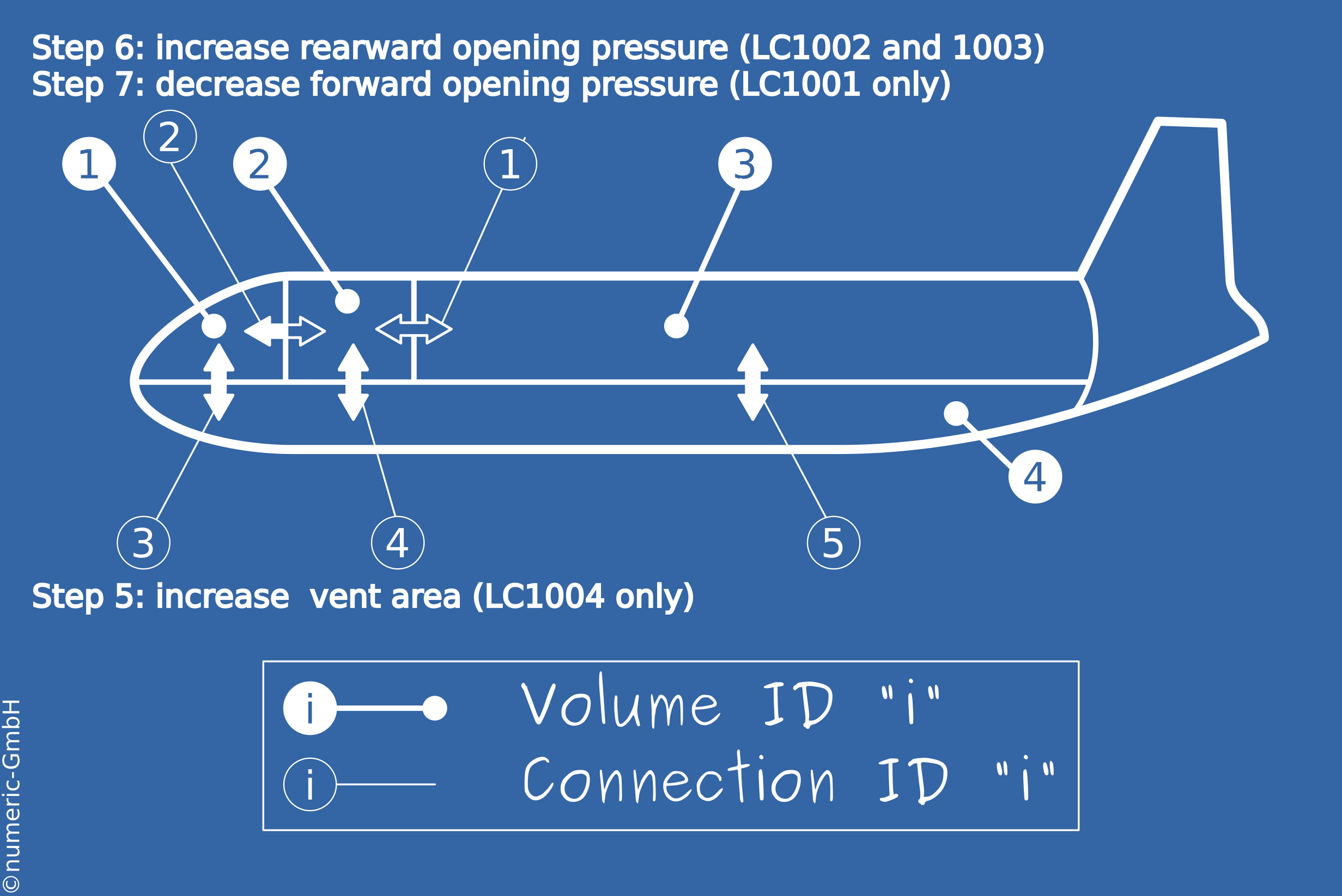
Fig. 9.61 problem 2 - Overview of the tweaked parameters

Running the Problem 2 and checking results¶

The user is invited to run the new model ESonix_tuto6c.xlsx creating the Node A4 of Tutorial #6.

Running a Sensitivity analysis between Node A3 (Reference model) and Node A4 (model modified with TWEAKS parameters) is an useful way of verifying the modifications introduced by the Tweaked parameters. The user is then invited to run this Sensitivity analysis, creating the Node A5 of Tutorial #6.

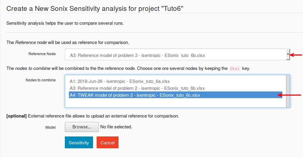
Fig. 9.62 Running Sensitivity Analysis between Nodes A3 and A4

In the results of Node A5 (Sensitivity A3/A4), the sections “Downloads” and “Overview” can be easily used to verify the modifications considered by the “tweaked parameters”.

Some of the possible analysis verification are shown below:

Modifications due to Step 5: In the Step 5, the Vent Area between main compartment and cargo was “tweaked” and its value increased by 10% for LC1004 only. Due to this modification a decrease of the downward floor pressure is achieved.

This result can be verified in the Bar chart of the “Cargo <> Main Deck” interface available in the “Overview” section.

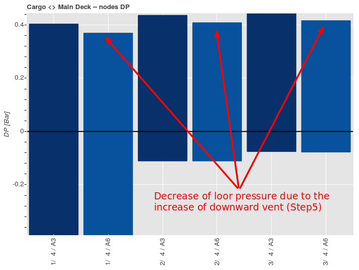
Fig. 9.63 Sensitivity A3/A4, LC1004 - Cargo to Main Deck Connections

Modifications due to Step 6: In the Step 6 the Opening Pressure between Vol1 and Vol2 was increased for load cases #2 and #3, which means that the opening of the vent area will be delayed and lead to an increase in the differential pressure between cockpit (Vol 1) and Entryway (Vol 2).

This result can be verified thanks to the Dynamic plotter accessible in the Sensitivity Analysis result page.

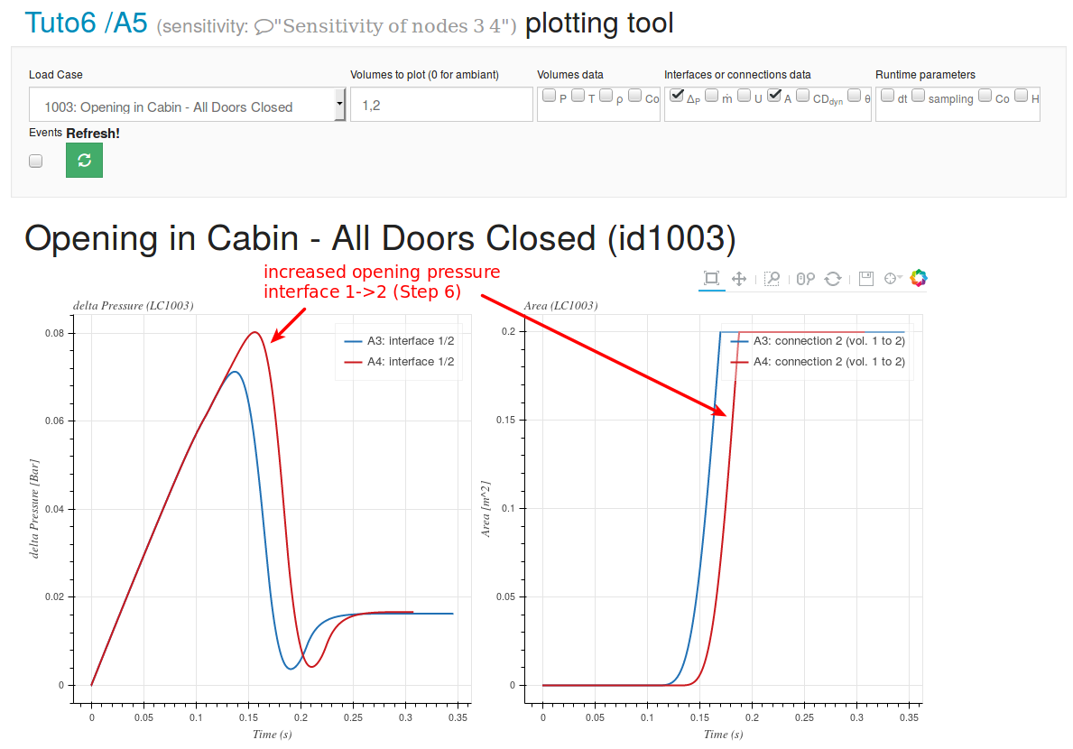
Fig. 9.64 Sensitivity A3/A4, LC1003 - Cockpit to Entryway Connection

Note

the effect of this modification is barely noticeable for the load case LC1002 as the cockpit door will open only 1.1ms later due to the pressure increase compared to 21.8ms impact on LC1003. The opening time info can be consulted in the “Events chronology” spreadsheet.

Modifications due to Step 7: In Step 7, the Opening Pressure between Vol2 and Vol1 was decreased for load cases #1 leading to a logical decrease in differencial pressure on the cockpit door and cockpit bulkhead. This effect can be verified in “DeltaP envelops spreadsheet”.

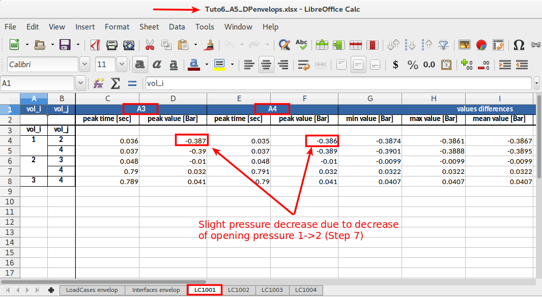
Fig. 9.65 Sensitivity A3/A4, LC1001 - Cockpit to Entryway Connection

Conclusion¶

Through this tutorial the implementation mechanism of the TWEAK parameters was presented.

The main goal of this tutorial was to show the versatility of the “TWEAK parameters”. Through “TWEAKs” the user can dynamically modify (tweak) an initial model in order to match some specific configurations seen on some of the load cases.

Another interesting way to use the “Tweaks facilities” is through trade-off studies in order to investigate the influence of a given parameter. Thanks to “Tweaks facilities” it is possible, for example, to investigate the influence of a connection Discharge Coefficient (Cd) on the differential pressures. (=> the same load case LC10xy should be repeated ‘n’ times in the load case definition sheet and then in the Tweaks sheet, the discharge coefficient will vary for each of those repeated load cases). The use of TWEAKs parameters offer a very powerful tool for detailed studies and complex decompression modelling.

Downloads¶

You can download the models used throughout this tutorial here under: