6. Analysis

ESonix features three kind of analysis:

• Regular
• Combination
• Sensitivity
• Batch

In addition to the analysis, the Tweaks facility is also available.

6.1. Regular runs

Regular runs are the basic analysis in ESonix. Once a project features several regular runs, the user can perform combination or sensitivity analysis on the top of them.

Model Initialisation

Once the model is uploaded on the ESonix Server, ESonix will perform several steps before triggering the run. This phase is called “Initialisation” and is described in Fig. 6.1.

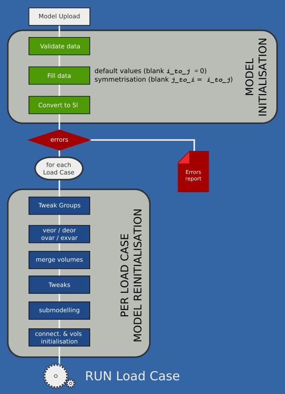
Fig. 6.1 Regular Run Model Initialisation Flow Graph

Preparation

A regular run is prepared and run from its father project by clicking on the new run, button as shown in Fig. 3.7.

The “new run” form is pre-filled with parameters defined during the Project creation (Creating a project).

Model parameters

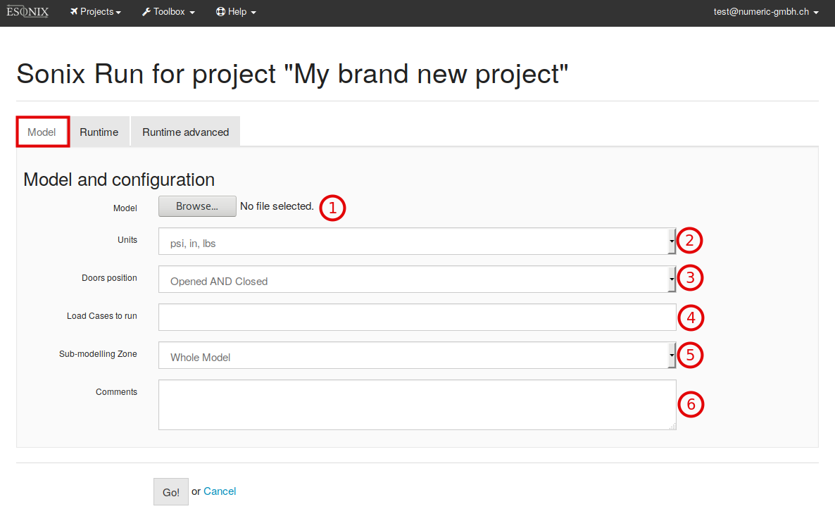
Fig. 6.2 New run model parameters Form

Model parameters are (numbers refer to Fig. 6.2):

1. Model: Button to browse and attach the XLS/XLSX model file to run.
2. Model’s Units system.
3. Doors Configuration to run.
4. Load Cases to run. Default (blank) is A
5. Sub-modelling Zone.
6. Comments: Free text. If blank, ESonix will fill it with miscellaneous data.

Runtime Parameters

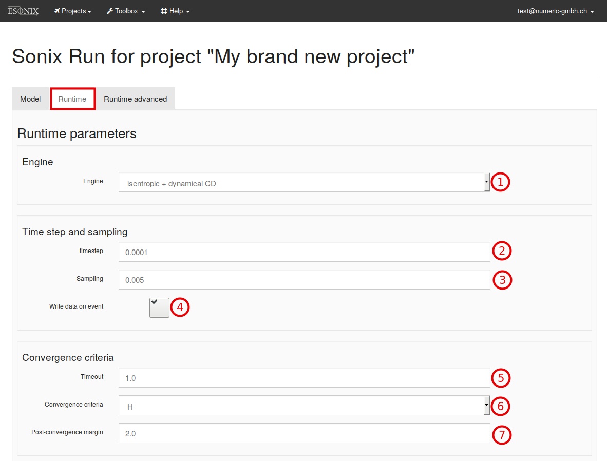
Fig. 6.3 New run runtime parameters Form

Runtime parameters are (numbers refer to Fig. 6.3):

1. Thermodynamical model (or engine).
2. Simulation time Step.
3. Simulation sampling.
4. Write Data on Event.
5. Simulation timeout.
6. Simulation Convergence Criteria.
7. Post-Convergence margin.

Runtime advanced Settings

Fig. 6.4 New run runtime advanced Form

Runtime advanced parameters are (numbers refer to Fig. 6.4):

1. adaptive strategy
2. adaptive strategy max co target
3. adaptive strategy neighborhood zone
4. adaptive strategy max co ramp
5. default opening latency
6. raw merging

Launch and evolution of the run

Once Go! button is pressed, the spreadsheet is sent to the ESonix server, with the relevant parameters. The spreadsheet is preprocessed and checked. If it contains no errors, calculation is automatically fired.

6.2. Combination Analysis

Combination analysis provides a mean to combine some regular existing nodes. It can be run by clicking on the Combination button as shown in Fig. 6.5.

Combination will build a single set of result based on the provided existing nodes. For example, in the Fig. 6.5 the Node A6 is a combination between Nodes A4 and A5.

Fig. 6.5 Combination Run Access

To do so, ESonix will begin by creating a load case mapping. This mapping will renumber existing load cases to avoid clash between models. For example, a combination made of three nodes would be mapped as follows:

Table 6.1 Example of Combination Laod Cases mapping

combined Load Case	Node ID	LodCase ID
1001	A1	1001
1002		1002
1003		1003
1004	A2	1001
1005		1002
1006	A3	1001
1007		1018

This can be read as follows:

Load Case 1005 for node A4 (combination of A1, A2 and A3) is actually load case 1002 from Node A2.

Once mapping is done, post-processing is performed in the same way as regular runs. All the tools available for regular runs are available for combination nodes, including sensitivity.

Opening in Cabin are usually checked with an empty cargo, such as an important mass of air is available in the cargo to be discharged into the cabin. At opposite, when checking an explosion in the cargo itself, it will be more conservative to assume a cargo occupied. Fig. 6.6 is extracted from Tutorial #4 illustrates the latter example.

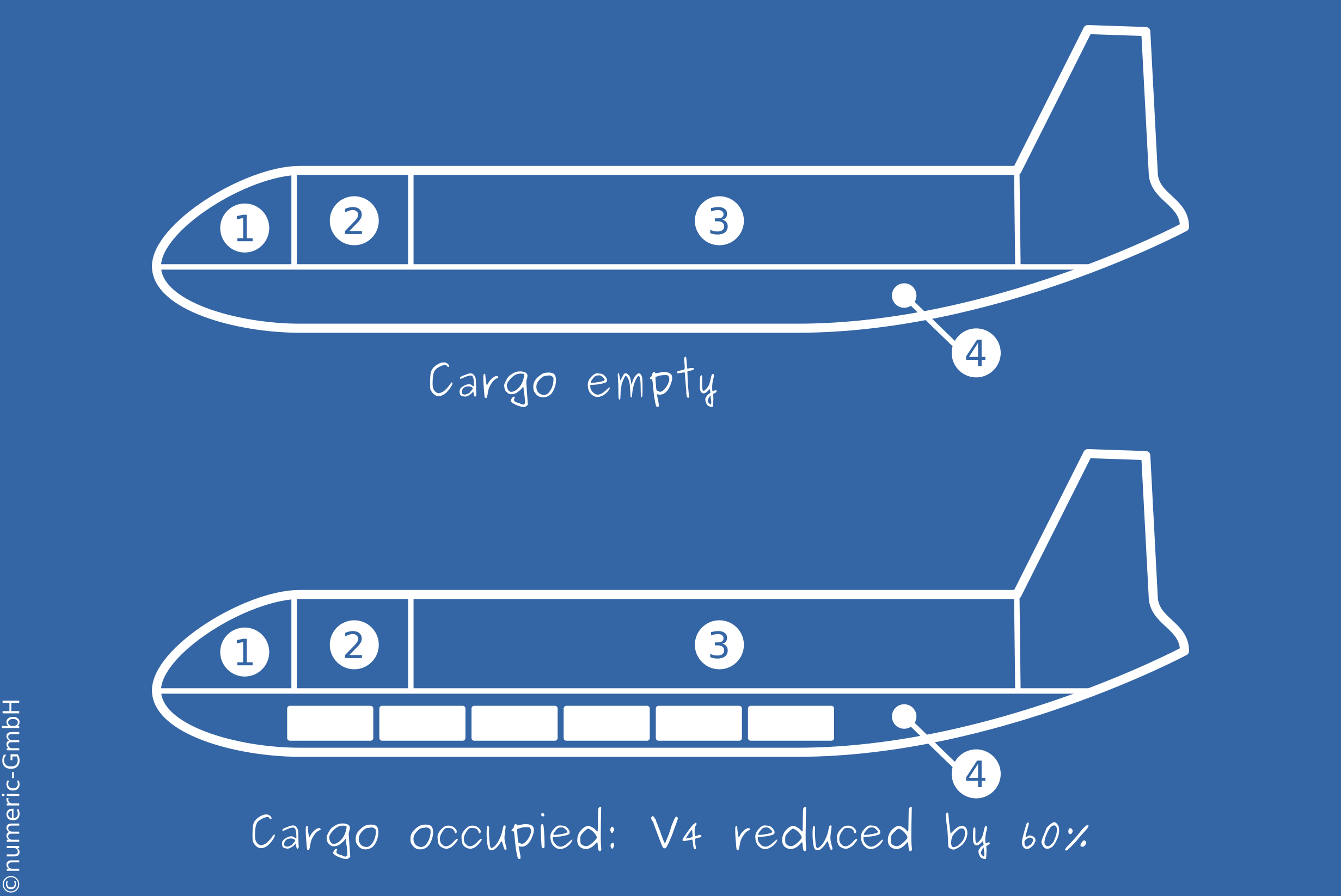
Fig. 6.6 Combination Analysis example

The example illustrated Fig. 6.6 could be addressed by combining two models: one with empty Cargo, one with occupied cargo. The first model would feature load cases for explosions in the main deck only (thus, volumes 1, 2 and 3), while the second one would feature explosion in the cargo (volume 4). The Load Case Mapping would then look like Table 6.2.

Table 6.2 Load Cases mapping relative to Fig. 6.6

combined Load Case	Node ID	LodCase ID	explosion in
1001	A1	1001	vol. 1
1002		1002	vol. 2
1003		1003	vol. 3
1004	A2	1001	vol. 4

See also

More details about combination analysis may be found in Tutorial #4.

6.3. Sensitivity Analysis

The sensitivity analysis gives the possibility to compare results between Nodes or between a Node and an external file. It can be run by clicking on the Sensitivity button as shown in Fig. 6.7. For example, in the Fig. 6.7 the Node A8 is a result of a sensitivity analysis between Nodes A6 and A7.

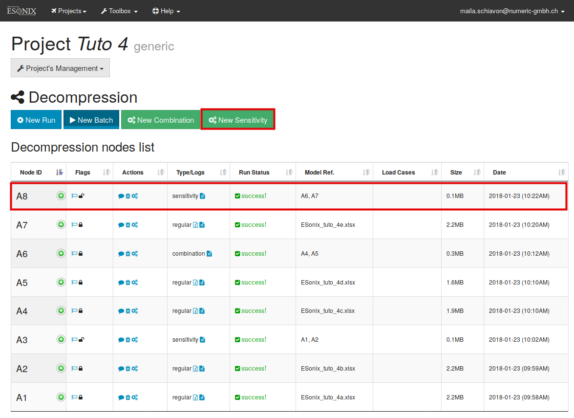
Fig. 6.7 Sensitivity Run Access

After clicking on Sensitivity button as per Fig. 6.7, the models need to be selected in the “Sensitivity Analysis Form” as per Fig. 6.8.

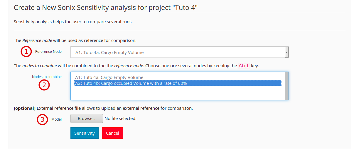
Fig. 6.8 Sensitivity Analysis Form

Sensitivity parameters are (numbers refer to Fig. 6.8):

1. Reference Node: Selection of the Node of reference.
2. Nodes to Combine: Selection of one or more nodes to be investigated.

3. Browse: option to run sensitivity analysis with external file (.xls/.xlsx). The ‘External File’ must be written as per a simple template as explained in (“External reference file”).

See also

More details about sensitivity analysis may be found in Tutorial #4.

6.4. Batch Analysis

The Batch analysis gives the possibility to:

• Run several Nodes in parallel.
• Enable easy parametric studies to check, for example, the influence of a set of parameters.
• Keep a organized back up of the Project giving the possibility of easily reproduce it.

Note

To run a Batch Analysis a Command File need to be previously written. This chapter explains how to write such a file.

The Batch analysis can be started by cliking in the New Batch button as per Fig. 6.9.

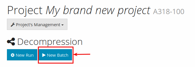
Fig. 6.9 Batch Access Buttom

After clicking on New Batch button as per Fig. 6.9, the files need to be uploaded in the “Batch Analysis Form” as per Fig. 6.10.

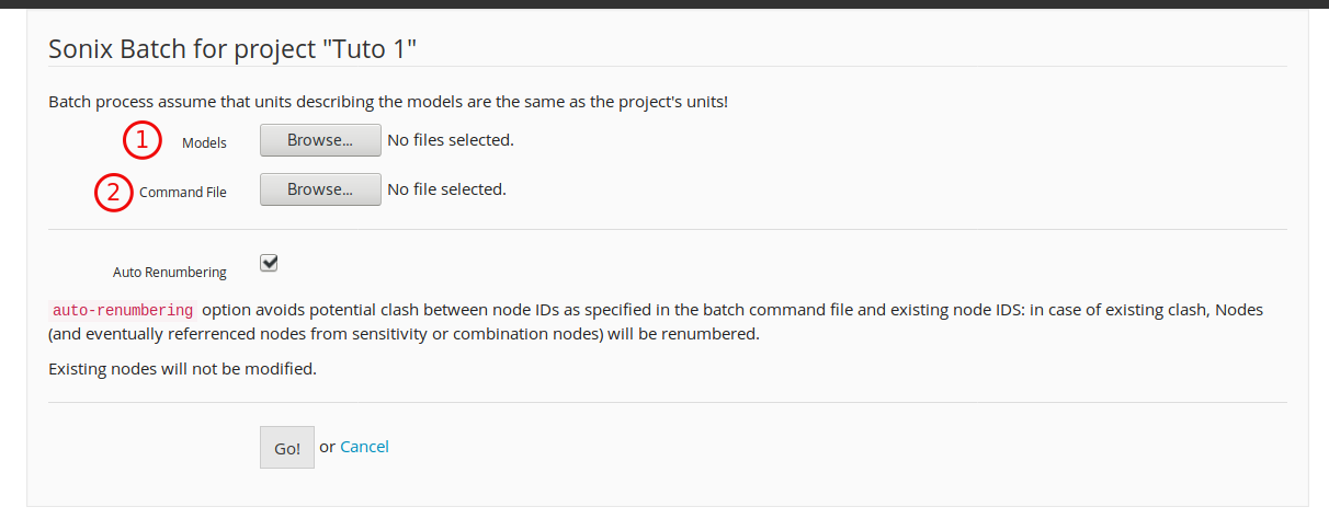
Fig. 6.10 Batch Analysis Form

Parameters are (numbers refer to Fig. 6.10):

1. Models: Selection of the Models (Excel spreadsheet) referred by the Batch Command File.
2. Command File: File describing all conditions (Node, Regular analysis, Sensitivity analysis, Combination Analysis, etc) to be considered in the Batch analysis.

Preparing the Command File

By the button Project Management two templates of Command File are available, as per Fig. 6.11:

• Batch Template: this template contains comments and general instructions to write a Command File. The use of this template is recommended for those starting with the Batch tool.
• Minified Batch Template: this template omits comments and instructions to write a Command File. The use of this template is recommended for those feeling comfortable with the Batch Tool.

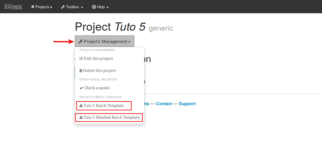
Fig. 6.11 Batch File - template access

As shown by the templates, three main sections may be considered in the Command File (numbers refer to Fig. 6.12):

1. [regular analysis]: where the default parameters and Models are defined.
2. [combination analysis]: where combination analysis between Models may be defined. This section can be deleted in case no combination analysis is required.
3. [sensitivity analysis]: where sensitivity analysis between Models may be defined. This section can be deleted in case no sensitivity analysis is required.

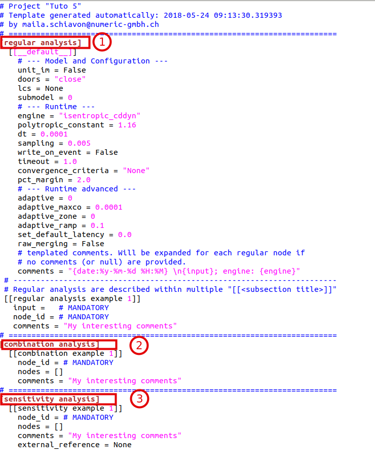
Fig. 6.12 Command File - Minified Template

Numbers refer to Fig. 6.12:

1. [regular analysis] section

The [regular analysis] subsection is divided in [__default__] subsection and models [regular analysis example 1, 2, 3, etc] subsection.

• [[__default__]] subsection

This subsection defines the main parameters for the analysis and default parameters for the regular nodes. It needs to be filled with the project’s default parameters as described in Model Parameters.

The [[__default__]] parameters are:

Model and Configuration

• Units
• Doors Position
• Load Cases to run
• Sub-modelling Zone

Runtime

• Engine
• Timestep
• Sampling
• Write Data on Event
• timeout
• convergence criteria
• Post-Convergence margin

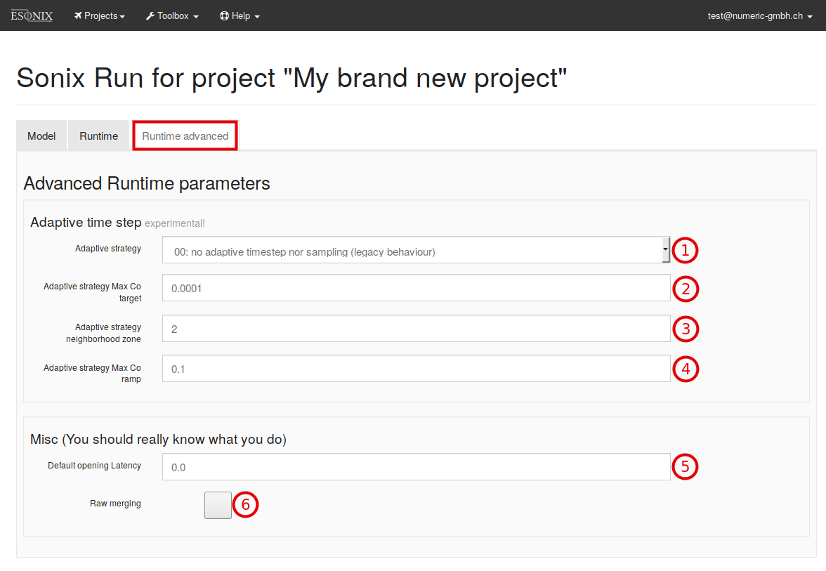
Runtime Advanced

• adaptive strategy
• adaptive strategy max co target
• adaptive strategy neighborhood zone
• adaptive strategy max co ramp
• default opening latency
• raw merging

.

• [[regular analysis example 1, 2, 3, etc]] subsection

In the [[regular analysis example 1, 2, 3, etc]] subsections (see Fig. 6.12 as reference), the Nodes need to be defined.

The parameters defined for each Node are:

• input: the input is the model (excell file tittle).
• node_id: Node identification.
• comments: to add any relevant comment.

Note

all parameters defined in the subsection [__default__] can be overlapped by new parameters for a specific Node if they are written inside the Node definition [regular analysis example 1, 2 3, etc].

2. [combination analysys] section

In this subsection (see Fig. 6.12 as reference), any kind of combination between the Nodes defined in the other subsections, can be requested.

• node_id: defines the identification of the combination node_id.
• nodes: defines the nodes that will be combined.
• comments: to add any relevant comments

3. [sensitivity analysys] section

In this subsection (see Fig. 6.12 as reference), any kind of sensitivity between the Nodes defined in the other subsections, can be requested.

• node_id: defines the identification of the combination node_id.
• nodes: defines the nodes that will be combined.
• comments: to add any relevant comments

See also

More details about batch analysis may be found in Tutorial #5.

6.5. Tweaks Facility

The Tweaks facilities allows the user to modify (tweak) pre-defined parameters as: volume, cp, vent area, etc. It is acessible via excell sheet called Tweaks. The Tweaks excell sheet is available in the Advanced Template, see Fig. 6.13 and Fig. 6.14

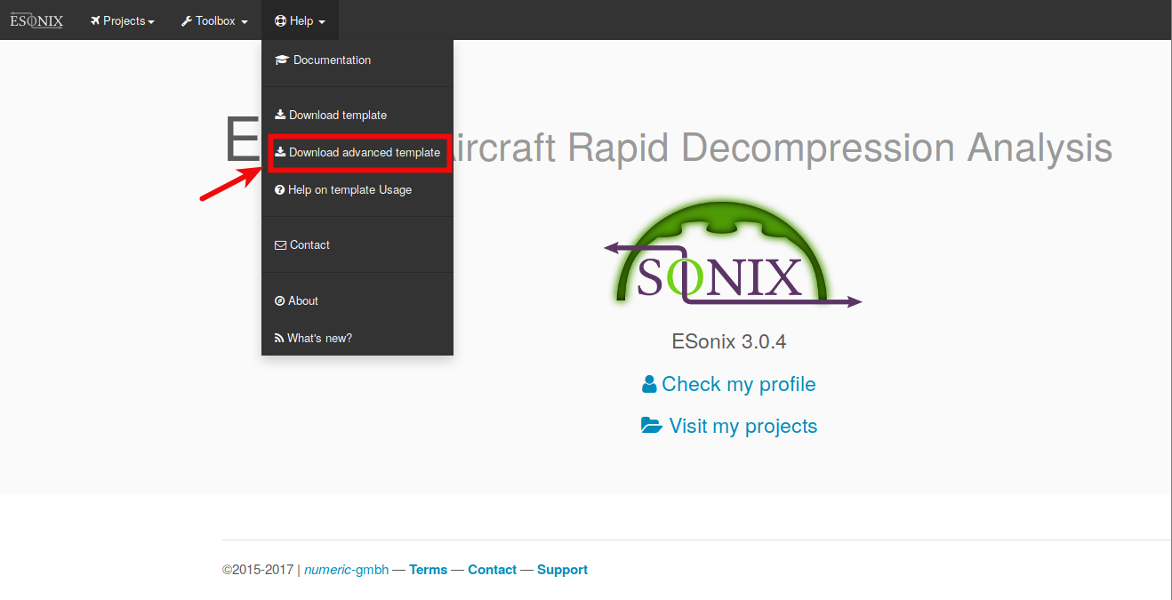
Fig. 6.13 Advanced Template - Download

The Fig. 6.14 shows the Tweaks excell sheet to ben considered.

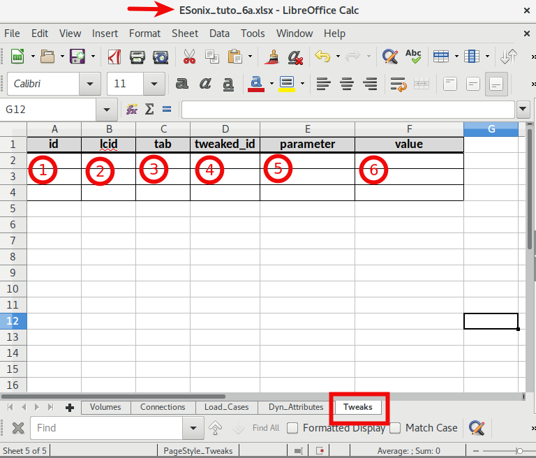
Fig. 6.14 Tweaks Excell Sheet

The numbers below refer to Fig. 6.14)

1. id : this column identifies the tweaked parameter(s).
2. lcid: this column identifies the load case id that will be considered for the tweaked parameter(s).
3. tab: this column identifies the reference tab that the tweaked parameter(s) will be considered.
4. tweaked_id: this column identifies inside the tab selected, the corresponding id of the tweaked parameter(s).
5. parameter: this column identifies inside the tab selected, the corresponding column of the tweaked parameter(s).
6. value: to add the value that should be considered by the Tweaks facility.

See also

More details about tweaks facility may be found in Tutorial #6.

6.6. Adaptive Runtime parameters

Courant number

As for ESonix3, ESonix is able to adapt the time step during run time. This means that the ESonix controller will increase time step when the model does not change quickly, and will decrease time step when the model is evolving quickly.

The actual value that ESonix is tracking is the volume’s courant number. For each volume i, this positive number is the absolute mass flow balance divided by the volume’s mass:

\[{Co}_i = \frac{\left | \Sigma \dot{m}_{ij}\right | }{m_i} \geqslant 0\]

With big mass flow balance (e.g. the volume is loosing a lot of hair compaired to its volume), the courant number will increase rapidly, and the simulation’s controller can decrease the time step to capture the event in a smooth way.

Volume neighborhood zone (neighborhood)

When defining an adaptive time step, it is important to specify the checked zone, or checked neighborhood. This zone defines where the Courant numbers will be checked.

The Maximum Courant number is the maximum of all or part of the model’s volumes Co. At a given instant, the volume having the biggest Co is the volume that is changing in a fastest way. We can therefore assume that connections attached to this volume are the one where the pressure differential \(\Delta_p\) is becoming critical.

The Controller will adapt the time step as follows:

\[\Delta T_{i+1} = B \cdot \Delta T_i \frac{Co_{target}}{Co_{max}}\]

where:

• \(B\): dumping coefficient
• \(\Delta T_{i}\): time step at instant i
• \(\Delta T_{i+1}\): time step at instant i+1
• \(Co_{target}\): Max courant number target
• \(Co_{max}\): Max courant number observed within the checked volume neighborhood zone.