8. Tutorials¶
This section aims to provide easy and stepping tutorials.
8.1. Tutorial #1¶
To get a primer to ESonix, nothing better than a fast & easy tutorial. This will help you to get the main concepts.
Introduction¶
We will run a really basic layout made of three equal volumes (v1, v2 and v3) connected by two passive vents (cf. Fig. 8.1)
We will simulate an explosion in volume 1.
Main assumptions:
- Internal pressure: \(1\ bar\)
- Ambient pressure: \(0.2\ bar\)
- Discharge Coefficients: \(CD=0.5\)
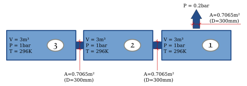
Fig. 8.1 Aircraft Layout
Create the model¶
Step 1: Download the model template¶
A decompression model is a simple Excel spreadsheet. You can start from a blank one although we advice to download a template from our site. You have an easy access from the menu bar, as shown in Fig. 8.2).
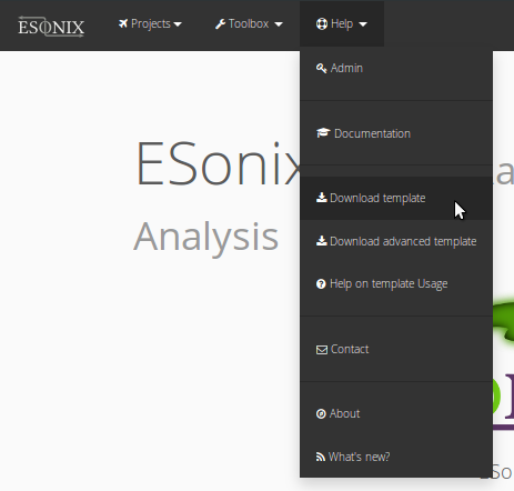
Fig. 8.2 Download Template
Save it on your own disk. You can (and you should) rename it. Let’s call it “ESonix_tuto_0.xlsx”.
Step 2: Define the Volumes¶
Edit the file with any Excel-compatible tool, and select the tab “Volumes”.
Fill in the first row with The First Volume (the one on the right on the previous schema) data, i.e:
id: 1volume: 3label: “Volume 1”deck: 0sta: 1rbl: 0
Now, go ahead with the two last volumes. Expected tab is shown Fig. 8.3.
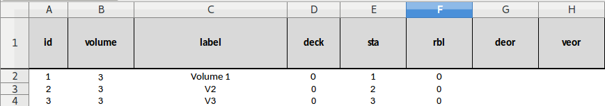
Fig. 8.3 Volumes Definition
The only differences between the rows shown Fig. 8.3 are (apart the labels) the sta values. We put here some dummy values that describe the geometric positions of each volumes.
Columns deck, sta and rbl need a bit of explanations: their values have no impact on calculations results. They are actually used only for post-processing stuff like organizing results into relevant sections or drawing A/C layout in a comprehensive way.
By using our template, you will have access to basic data control (try
to enter some text in the volume columns). Additionally, some useful
data are provided via tool tips.
Now the next step is to define the connections.
Step 3: Define the Connections¶
This is usually the most tricky part, although it will go smoothly for our current example.
As defined in Fig. 8.1, we have two connections in this model. Let’s define them as:
- Connection #1: Passive vent between Volume 1 and Volume 2, area=0.07065m², CD=0.5
- Connection #2: Passive vent between Volume 2 and Volume 3, area=0.07065m², CD=0.5
A “passive vent” is called passive by opposition to “featured vent” or “active vent”. A “passive vent” is a simple opening that is always opened , like Toe-kick grids.
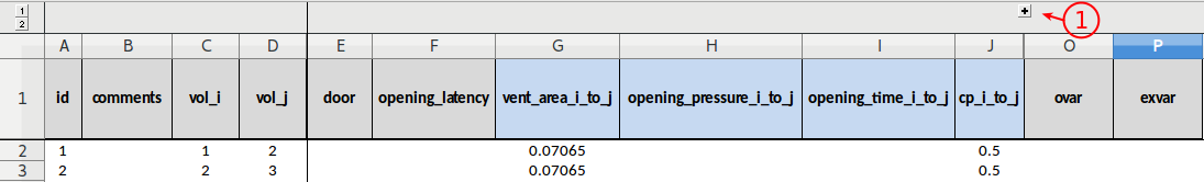
Fig. 8.4 Connections Definition
Note
Observe in Fig. 8.4 how we filled only the
relevant fields. The “*_i_to_j” columns
(highlighted in Blue in the ESonix Model template) will be interpreted
to be zero when empty. ESonix will therefore assume that opening time
is \(0\ sec.\) and opening pressure is \(0\ psi\): the
connection is always opened for any pressure.
The “*_j_to_i” parameters are highlighted in Red in the ESonix Model
template, and folded by default. You can access them by unfolding the
group (item #1 on Fig. 8.4).
We will actually let them as they are since ESonix will assume that
values are the same than “*_i_to_j” values. Here come two major tips:
- Any Empty value in the
i_to_jcolumns will be interpreted as “zero”. This is called initialisation phase. - Any Empty value in the
j_to_icolumns will be internally copied from thei_to_jvalue. This is called symmetrization phase.
See also
Refer to model connections Preprocessing for detailed informations about connections initialisation.
The next step is to define the Load Cases.
Step 4: Define the Load Cases¶
The last modifications we will perform on our model is to define the so-called load cases. A load case in the decompression process is an opening from the cabin to the ambient.
The tab used for this purpose is titled “Load_Cases”
What defines a load case in last resort is therefore:
- Where is the hole opening? Which volume will be connected to the Ambient?
- Which size the opening hole is?
- Which discharge Coefficient to use?
- Which conditions in the cabin (Pressure and Temperature)
- Which conditions in the ambient (Pressure)
The answers to this questions are given by the regulations (e.g FAR 25.365e for the opening holes)
For our tutorial, we will create a single dummy load case:
Opening in Volume 1 with a size equal to internal vents. A discharge Coefficient of 0.5 will be used. Pressure in the cabin is \(1\ bar\) whereas pressure in the ambient will be taken equal to \(0.2\ bar\).
Model you should get is shown Fig. 8.5.
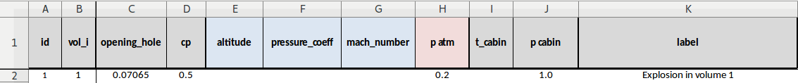
Fig. 8.5 load cases Definition
And that’s it for our model! The next step will consist in creating a new Project on the ESonix platform.
Run your model¶
If you do not have any account on ESonix, it’s time now to create it!
If you are not logged in, well, it’s also time to do it.
Step 5: Create a project¶
Once identified on the platform, create a new project from the top bar (cf. Creating a project).
Fill in the form. Call the project “tuto1” (Fig. 8.6)

Fig. 8.6 project Definition
Modify default values as follows:
- Name
- A/C type
- Set units to “bar, m, kg”, such as ESonix is aware about how is described the model
- Set the engine to isentropic
- Set doors configuration to “Closed”
Note
The A/C type field should normally content the Aircraft type, like A319 or B777.
For the current tutorial, Doors position actually doesn’t matter
since we do not have doors in the model. You may have chosen
“Opened”, it wouldn’t have changed the calculations. “Opened and
Closed” is useful for real-life models with actual doors installed
where we need to simulate both configurations.
Once you saved, you will be redirected to your new project central page.
Step 6: launch your analysis¶
Click on the New Run button. You will be redirected to a form
(Fig. 8.7).
From this form, select your spreadsheet. All the other parameters have been defined as default parameters from the model.

Fig. 8.7 New Run Form
Once you clicked on “Go!”, calculations are performed.
Check the results: the “results” page¶
See also
Only a few limited tools are presented hereunder. Refer to Post processing for much more details.
Once calculations are performed, you will be redirected to the results page. Several sections are available, including:
“Downloads” Section¶
This section provides several spreadsheet as deliveries, such as Δp envelops, events chronologies, etc.
Curves plottings¶
You can plot different kind of values against time by following the appropriate link “dynamic plotter”. For example, let say you wish to check the evolution of Pressure and delta-pressure between volumes 1 and 2 (Fig. 8.8)
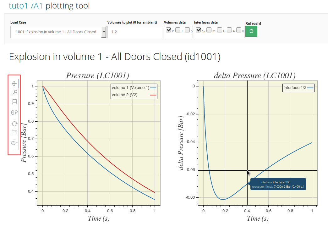
Fig. 8.8 Plotting variables over time using the dynamic plotter
Plots are dynamic: you can move the mouse over the curves to get data. But you can also zoom on the figures by scrolling the mid-button.
Conclusion¶
You learnt through out this tutorial the basics to prepare, run and check a very basic model.
You can download this model from here:
8.2. Tutorial #2¶
We will start from the model created for the Tutorial #1.
You can download this model from here: http://www.aero-sonix.com/static/support/ESonix_tuto_1.xlsx
This model idealizes its two internal vents as passive vents, i.e venting area is constant over time.
To go one step forward, we will now learn how to idealize active vents such as decompression panels, and how to create multi-load case analysis.
Node A1: Same model, 3 load cases¶
To get some more fun, we will first introduce a multi-load case analysis by adding two additional load cases to the first model.
Rename the previous model to “ESonix_tuto_2a.xlsx”. Edit it to reflect the following proposal:
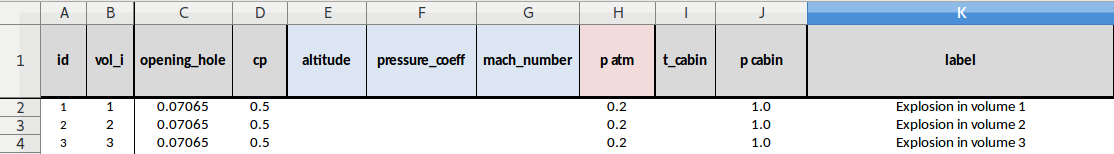
Fig. 8.9 load cases Definition
We basically created three load-cases: each of it simulating an opening in a different volume.
Create a project “tuto 2”. To have a reference to compare our next runs, let’s run this model with the same parameters as the ones used in tuto#0.
Warning
Watch the units! When defining the new run, take care to specify the correct units! The correct ones for this tutorial are “bar, m, kg”.
Node A1: explore some of the Esonix pages¶
The node results page¶
You will be redirected to the results page. Find the Overview section, and unfold the panel “Main Deck to Main Deck”.
Two graphs are shown there:
- a heatmap showing the maximum absolute value for each load case and each defined interface.
- a bar plot summarizing the max values for both directions for each interface.
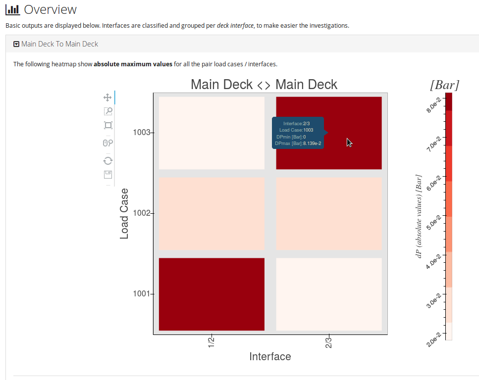
Fig. 8.10 Main deck to main deck heatmap

Fig. 8.11 Main deck to main deck histogram
Warning
Interface definitions and sign of \(\Delta_P\)
From the last figure, we can check that the maximum \(\Delta_P\) for interface “1/2” is \(+0.081\ bar\) for pressure acting from 2 to 1, and \(+0.02\ bar\) for pressure acting from 1 to 2.
The project page¶
From the previous run results page, you can go back to the project by clicking on the project name, at the top of the page.
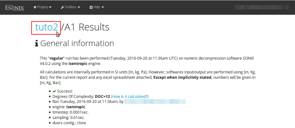
Fig. 8.12 Back to the project main page
From there, you can see that a “Decompression nodes list” was created. Here will be tabulated all the runs you will perform for a given project.
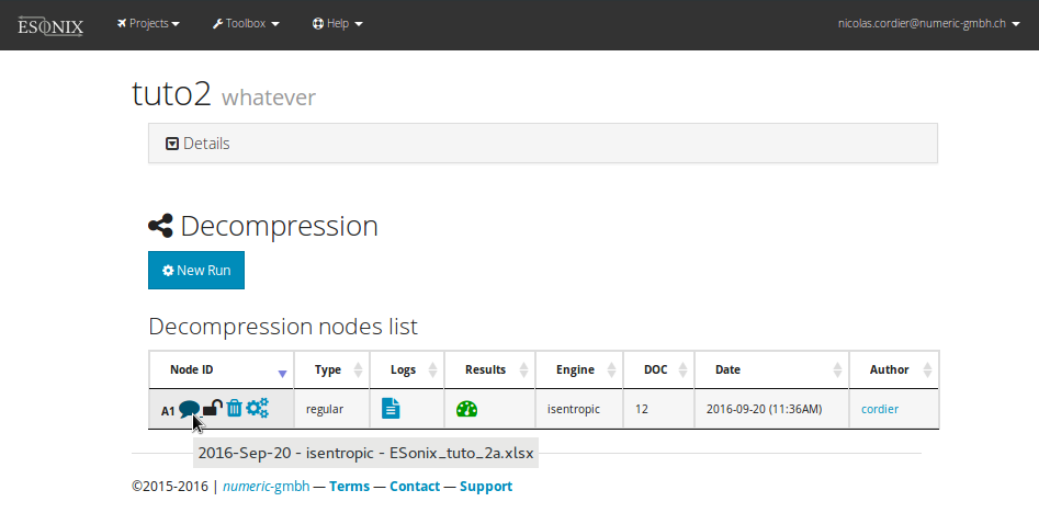
Fig. 8.13 Project nodes list
Let’s go quickly trough the line to explain the symbols. Some of them will show some useful tooltips when hovered.
Fig. 8.14 Project nodes list Icons
Column Node ID¶
The columns shown in :numerf:tuto2_icons are:
- Node ID (“A1”). This node ID is the identification number for this run .The next run will be called “A2”, etc.
- Comments symbol: By clicking on it, you can append some comments to your run. This helps to keep track of important informations.
- Lock: An analysis cannot be deleted if the lock is “on”.
- Trash: Click on it to delete the files.
- Postprocess: Click on it to redo post-processing. Usually not useful except after an update of the software to gain access to an eventual new feature.
- Type of analysis (here is “regular”). Different kind of analysis can be run. The simplest one is identified as “regular”. You can have as well “combinations” and comparisons” analysis.
- Shortcut to Analysis logs.
- Access to the results main page. Green if the run was fine, red if something bad happened and no results are available.
- Engine used for the analysis.
- Degree of Complexity (doc).
- Run date and time (server time – UTC+1).
- Author of the run (hyperlink to email address)
Node A2: Decompression panel¶
In place of the current passive vent between volumes 2 and 3, we now have to simulate a decompression panel with the following characteristics:
- Full frame Area = \(0.07065\ m^2\) (as before)
- Opening time = \(0.2\ sec.\) to get the full area.
- Pressure release = \(0.15\ bar\)
- The panel is supposed to open in both directions.
Copy your “ESonix_tuto_2a.xlsx” to “ESonix_tuto_2b.xlsx”, and edit it to reflect this:
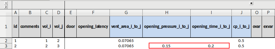
Fig. 8.15 Defining connections for decompression panel
Since the panel is supposed to have the same characteristics for both
directions (from volume 2 to 3 and from volume 3 to 2), no need to edit
the j_to_i columns: they will be automatically copied from the
i_to_j columns.
From the A2 results page, go to the “overview” section as before, and compare the results we have now compared to A1.
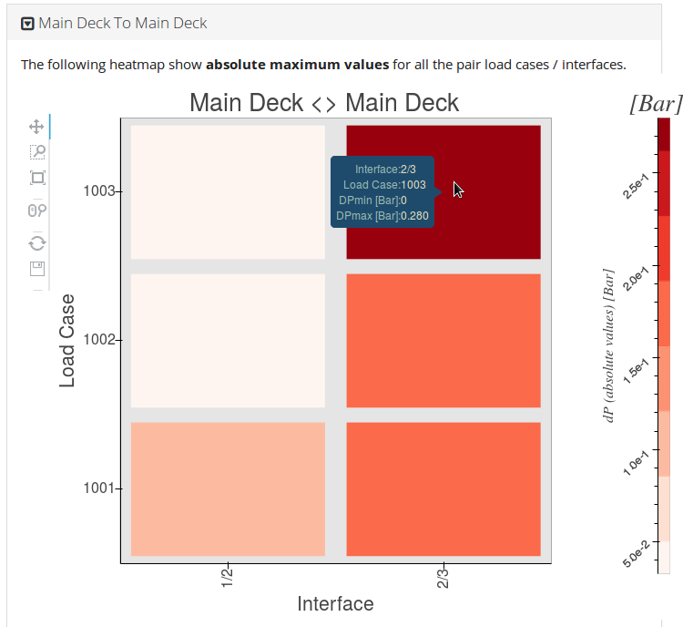
Fig. 8.16 A2 main deck to main deck Heatmap
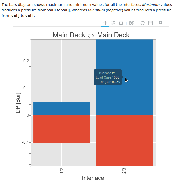
Fig. 8.17 A2 main deck to main deck histogram
Whereas results were “symmetric” for node A1, the decompression panel we introduced decreased maximum pressure that interface 1/2 was reacting, and increased the maximum pressure the interface 2/3 reacts, whatever the direction we check.
We can go one step further and investigate what happens with interface 2/3: click on the “Dynamic plotter”, as shown in Fig. 8.18.
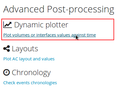
Fig. 8.18 dynamic plotter hyperlink
We will plot \(\Delta_P\) and \(Area\) for interfaces “1/2” and “2/3” for load case 1003, as shown in Fig. 8.19.
Select:
- Load Case: 1003
- Volumes to plot: enter “1,2,2,3”, to be understood as 1/2, 2/3
- Values to plot: check “Δp” and “A” (delta pressure and Area)
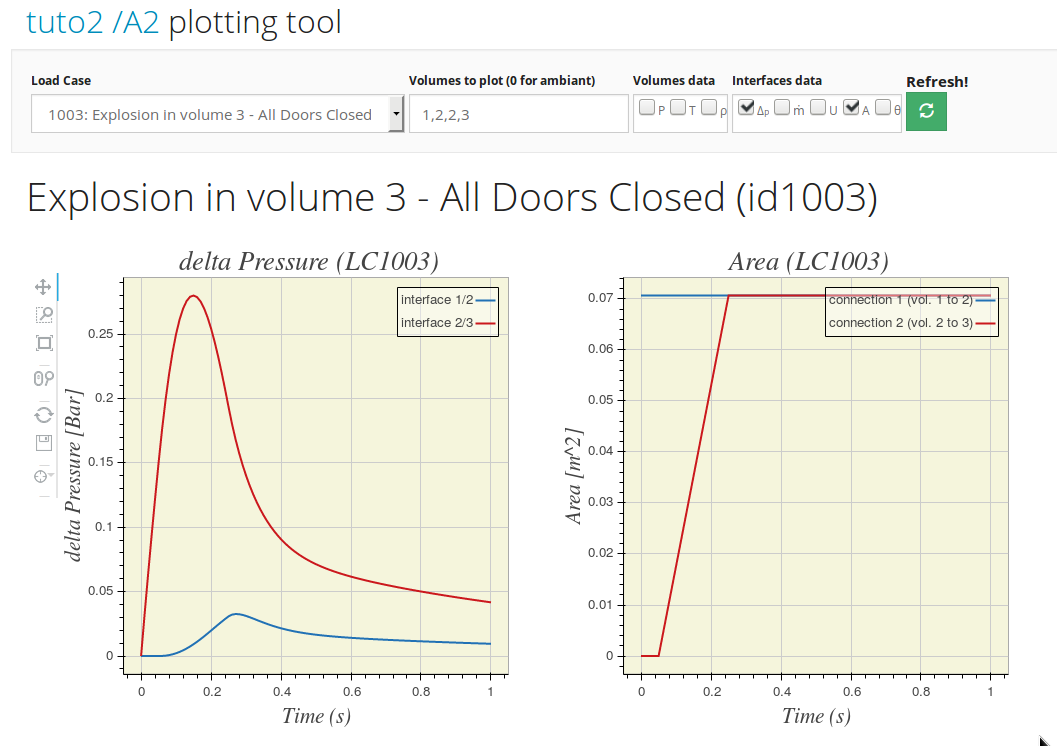
Fig. 8.19 Curves for interfaces 1/2 and 2/3
From the Area curves (on the right), it is clear that connection ID2 starts to open around 0.04 second, which is the time where \(\Delta_{P\ 2/3}\) reaches the released pressure (\(0.15\ bar\)).
DeltaP values from XLS results files¶
You can double check this opening behavior from the “download section”.
Go back to the A2 results page (Fig. 8.20)and download the Δp spreadsheet (Fig. 8.21).
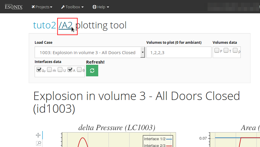
Fig. 8.20 Back to node’s main page!
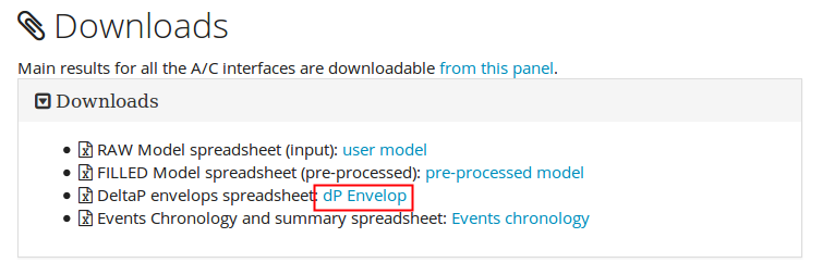
Fig. 8.21 Download node A2’s Δp spreadsheet
The first tab from the XLS files is titled Interfaces envelop and shows the envelop by interface (Fig. 8.22).

Fig. 8.22 per interface Δp envelop tab
The max \(\Delta_P\) for interface 2/3 is thus \(0.28\ bar\)
(column absmax_v), occurring at \(0.1501\ sec\) (column
absmax_t) and for load case 1003 (column lcid_absmax)
The second tab from the XLS files is titled LoadCase envelop and shows the envelop by load case. We highlighted in Fig. 8.23 the envelops for load case 1003.
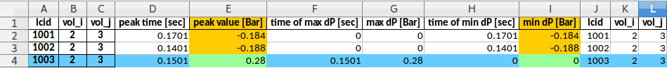
Fig. 8.23 per load-case Δp envelop tab
As expected, the max value highlighted from the by-load case envelop is the same as the highest value from the by-interface envelop.
Another interesting check is that the interface 2/3 is always critical, whatever the load case.
Chronology from XLS results files¶
Downloading the “Events chronology” spreadsheet provides summary to events occuring during the decompression.
From Fig. 8.24, we can double-check that the connection we defined with ID 2 (between volumes 2 and 3) is opening for a DeltaP=0.15 bars, and its opening is running for 0.2 seconds, from t=0.0501 seconds to t=0.2502 seconds.
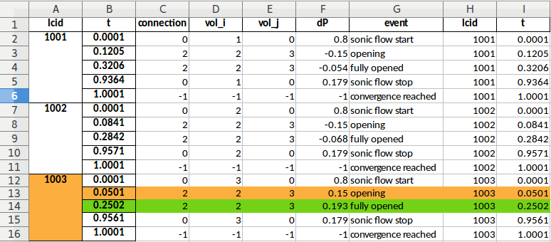
Fig. 8.24 Chronologies for all the load cases. Coloured lines highlight the opening of connection ID2 (0.2 seconds).
Downloads¶
You can download the models used through out this tutorial hereunder:
8.3. Tutorial #3¶
The Tutorial #1 referes to ESonix basics, Tutorial #2 explores basic decompression features definition, we will now explore how to define a door.
What is a “door” for ESonix?¶
Actually, a “door” as seen from ESonix, is not a decompression feature.
For ESonix, the concept of “door” is usefull to define a fully static vent that is either opened or closed, depending on the configuration ran.
From the ESonix Excel template file, you can tag a connection as “door”
by filling the “door” column. If a connection is identified as a
door by ESonix, the corresponding path area will be cleaned when ESonix
runs an “Opened door configuration” run. Obviously, the path will be
closed for a “Closed door configuration”.
That being said, a door can act:
- as a full decompression feature (e.g.: swivel doors) if the
“
vent_area_*” has the same value as the “door” column value. - as a nested decompression feature (e.g.: decompression panel) if
the “
vent_area_*” is lower than the “door” column value.
A connection tagged as “door” with a “vent_area_*” value equal to 0
will always be closed during a “Closed door configuration”.
Some more info can be found in the dedicated section doors, and in some useful common examples, like Simple decompressing door.
Defining a swivel door that doesn’t decompress: A1¶
To save some time, we will start from the second model created during the Tutorial #2. You can download this model from here: http://www.aero-sonix.com/static/support/ESonix_tuto_2b.xlsx, and save it as “Esonix_tuto_3a”.
In place of the current decompression feature between volumes 2 and 3, we now have to simulate a swivel door that does not decompress. All the other parameters remain the same:
- Full frame Area = \(0.07065\ m^2\) (a hobbit door, as before)
- Opening time = No need as the door does not decompress.
- Pressure release = No need.
- Discharge coefficient CP = 0.5
Fig. 8.25 shows the modified model spreadsheet.
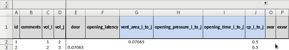
Fig. 8.25 Connection #2 is a simple non-decompressing door.
Connection ID2 is defined as “door” by filling the door column. Since the
door is not supposed to decompress, vent_area_i_to_j and
vent_area_j_to_i are set to zero (or let blank).
Run the simulation, for both opened and closed configurations¶
Create a new project called “tuto3”, preset it with appropriate units, and
select “Opened AND Closed” configuration.
The run the first node with the modified spreadsheet. Since you selected
“Opened AND Closed” and defined three load cases (one explosion per
compartiment), ESonix will therefore run six load cases:
- All doors closed, explosion in volumes 1: Load Case 1001
- All doors closed, explosion in volumes 2: Load Case 1002
- All doors closed, explosion in volumes 3: Load Case 1003
- All doors opened, explosion in volumes 1: Load Case 2001
- All doors opened, explosion in volumes 2: Load Case 2002
- All doors opened, explosion in volumes 3: Load Case 2003
Note
Load Cases numbering
ESonix will translate the Load Cases IDs defined from your model in two series:
- 1000 + Load Case ID for an “All Doors Closed” configuration
- 2000 + Load Case ID for an “All Doors Opened” configuration
Check the node A1’s results¶
What we may expect?¶
For the “Doors Opened” configurations (load cases 2001 to 2003), the problem is symmetric, and we expect \(\Delta_P\) for interface 1/2 and 3/2 need to be the same, as all the air path are equal.
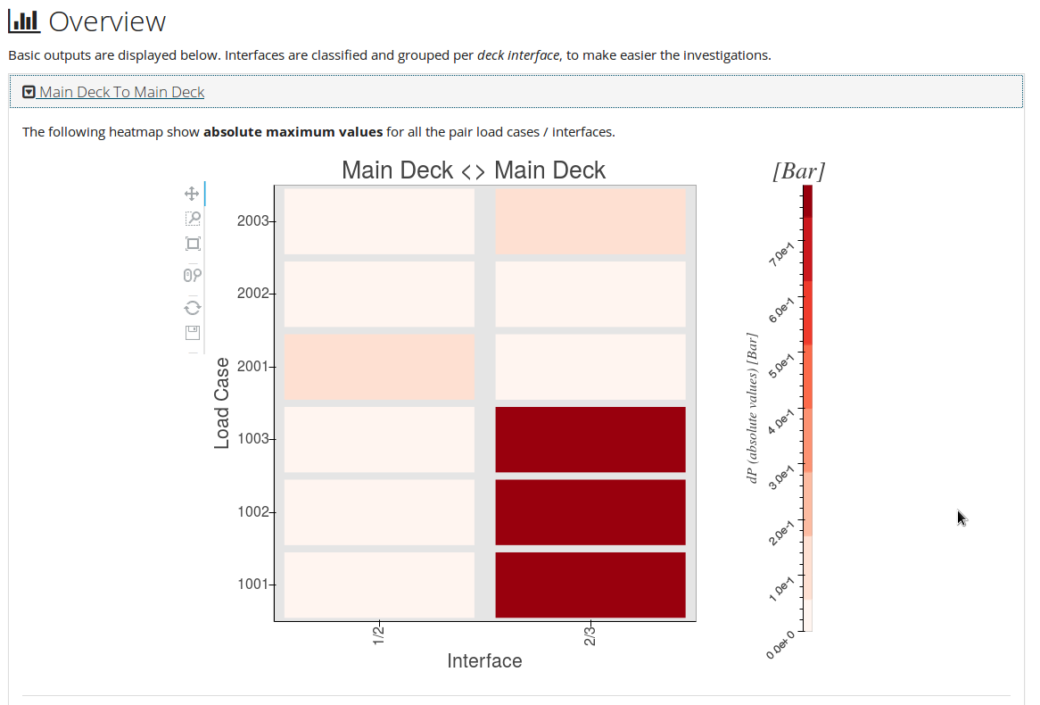
Fig. 8.26 Main deck to main deck A1 heatmap
For the “Doors Closed” configurations (load cases 1001 to 1003), the volume 3 will always be isolated from the rest of the cabin: the door will stay closed as no decompression feature is provided. Final Δp between volumes 2 and 3 should be equal to initial Δp between cabin and atmosphere (thus 0.8 bar).
This is the case for LC1003 only. For LCS 1001 and 1002 decompression time are longer than the 1 second assigned by default to the run (cf. advanced settings), and the air from volumes 1 and 2 has not fully exhausted to ambient.
Defining a decompressing swivel door: A2¶
We now want to change this door useless for decompression to a single-way decompressing swivel door. Let’s say we need a door opening at 0.15 bar, and reaching its full opening in 0.2 seconds (which is quite long).
In that purpose, we just need to specify an opening area equal to the door’s frame (thus 0.07065 m²), as the full door is opening.
Copy your initial file to “ESonix_tuto_3b.xlsx”, and change the “Connections” tab to match Fig. 8.27.
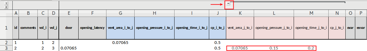
Fig. 8.27 Connection #2 is a swivel decompressing door.
Since we want the door to open from volume 3 to volume 2, we need to
specify the values for the j_to_i columns. Discharge coefficients
CP is valid for both ways, and specify it in the i_to_j columns
is enough: it will be copied to the j_to_i values. It would have
been ok though to specify it again.
Launch the run as before, and check this new set of results (should be node A2).
Check the node A2’s results¶
What we may expect?¶
The most obvious result we expect is for an explosion in volume 3 and all doors closed: since the door is opening from 3 to 2, the door should never open, and maximum \(\Delta_{P\ 2,3}\) should be equal to initial \(\Delta_P\) between cabin and atmosphere (thus \(0.8\ bar\)).
We can easily check it from the heatmap Fig. 8.28.
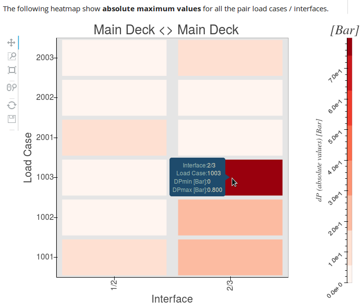
Fig. 8.28 Main deck to main deck A2 heatmap
We could also check it from the curves tool by plotting the venting area for interfaces 1,2 and 2,3 and for load case 1003 (Fig. 8.29).
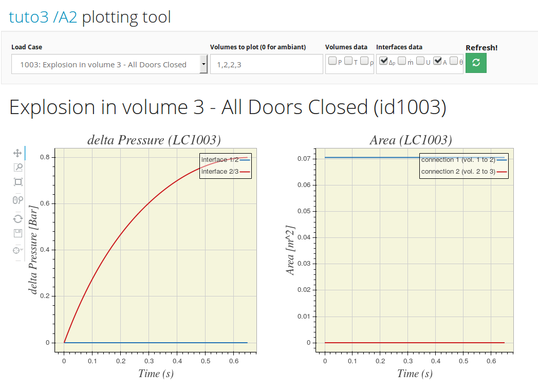
Fig. 8.29 A2 Δp and Area for interfaces 1/2 and 2/3 for load case 1003
It is clear from the Fig. 8.29 that area for interface 2,3 remains 0, and that \(\Delta_{P\ 2,3}\) converges to \(0.8\ bar\).
If we plot the same data but for Load Case 1002 (explosion in volume 2 for an initial cabin configured with all doors closed, we can expect the door to open in the defined 2 seconds, and \(\Delta_{P\ 2,3}\) converges to \(0\ bar\). This is shown Fig. 8.30.
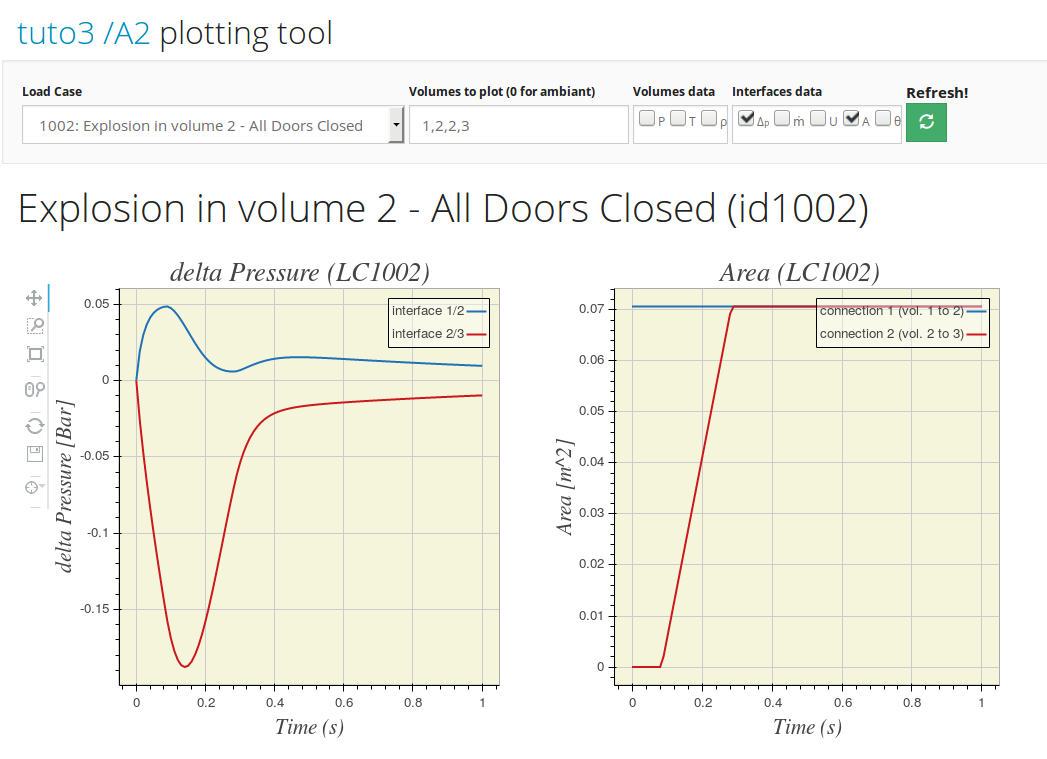
Fig. 8.30 A2 Δp and Area for interfaces 1/2 and 2/3 for load case 1002
Defining a door hosting a decompression panel: A3¶
If the same swivel door as defined above would feature a decompression panel, assuming the decompression panel (let say a 0.03m²) opens in both directions, the door would have to be defined as follows:
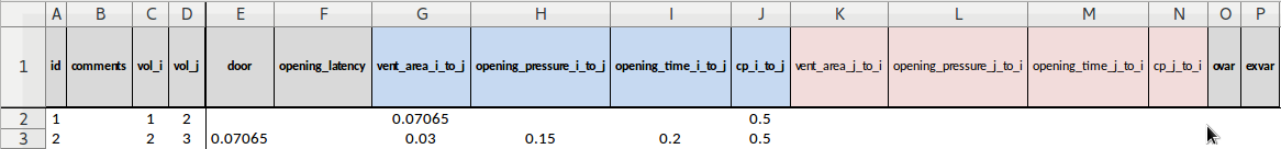
Fig. 8.31 Connection #2 is a swivel door hosting a nested decompression panel
Defining a decompressing swivel door with dynamical attributes: A4¶
We defined in Defining a decompressing swivel door: A2 (node A2) a decompressing swivel door. To simulate the time the door will use to completely open, we set an opening time equal to 0.2 seconds.
Defining the opening time for all decompressing features can be heavy, and will necessarily be an approximation as opening time depends on real pressure acting on the item.
As of ESonix version 2, dynamical attributes may be added on already defined
decompression items. Documentation tab “Dyn_Attributes” describes the way to
do so: it mainly consists in adding a new tab to the basic model: dyn_attributes.
The easiest way is to download the “advanced template” as proposed from the “help” menu (Fig. 8.32).
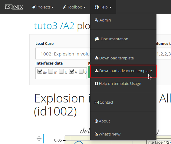
Fig. 8.32 Download the “advanced template” from the “help” menu
Copy the “Dyn_Attributes” tab to the spreadsheet used for node A2. This node was used to simulate swivel decompressing door.
Assuming the door will be a square panel with the same area as initial door, and a mass of 15kg, fill the Dyn_Attributes spreadsheet as shown in Fig. 8.33.

Fig. 8.33 Connection #2 is a swivel decompressing door with a dynamical behaviour.
See also
Current manual section tab “Dyn_Attributes” for complete reference about dynamical attributes parameters.
Downloads¶
You can download the models used through out this tutorial hereunder:
8.4. Tutorial #4¶
This tutorial starts a new example from scratch. It is however recommended to practice with tutorials Tutorial #1, Tutorial #2 and Tutorial #3 before training with this one.
Presentation of the problem¶
This tutorial is based on [PC16], §5.4 “Four-Compartment aircraft”.
It will be studied an Aircraft made of three volumes at the main deck and one single cargo (Fig. 8.34). To characterize the influence of an occupied cargo, two models will be studied:
- Cargo empty volume = 67m³ (model A)
- Cargo occupied with a rate of 60% occupancy (therfore, cargo volume =67m³-60% = 26.8 m³ (model B)
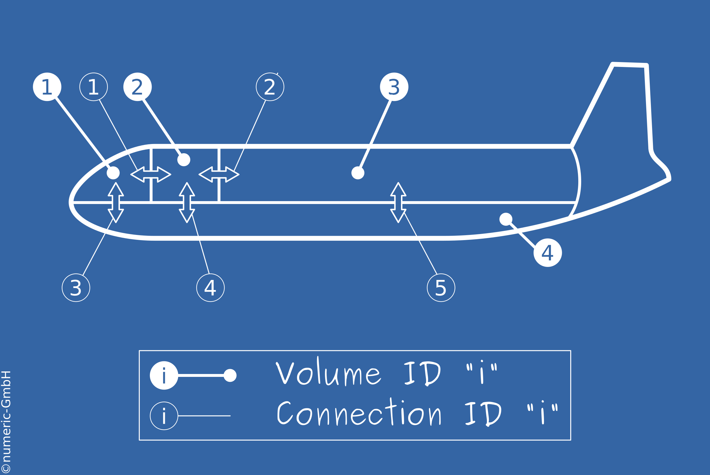
Fig. 8.34 Four volumes definition
Those two models will be ran to create two nodes A1 and A2. A sensitivity analysis will be performed on those two nodes to create node A3. This sensitivity analysis will be used to understand the influence of the cargo occupancy.
Once the critical configuration will be found using sensitivity analysis, we will create two models (A4 and A5) to be combined in a single set of results (node A6).
Lastly, a unified model will be created to show the basics of model unification (node A7).
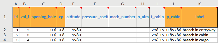
Empty Cargo Volumes definition (model A)¶
The following values will be used:
| ID | label | volume |
|---|---|---|
| 1 | Cockpit | 4m³ |
| 2 | Entryway | 3m³ |
| 3 | Cabin | 198m³ |
| 4 | Cargo empty | 67m³ |
Pressure cabin is given to 89.786 kPa (0.89786 bar), Temperature in the cabin is 23°C (296.15K)
Occupied Cargo Volumes definition (model B)¶
The volume of the cargo is reduced by 60%. New volume is therefore set to 26.8m³.
| ID | label | volume |
|---|---|---|
| 1 | Cockpit | 4m³ |
| 2 | Entryway | 3m³ |
| 3 | Cabin | 198m³ |
| 4 | Cargo occupied | 26.8m³ |
Same cabin pressure and temperature as model A are used.
Connections definition (models A and B)¶
For Both models (model A and model B), compartments are connected as follows:
| ID | type | vol_i | vol_j | length | width | release pressure | Discharge Coeff. | Weight |
|---|---|---|---|---|---|---|---|---|
| 1 | passive | 2 | 3 | 1.8 m | 0.5 m | na | 0.7 | na |
| 2 | Vertical hinged blowout | 1 | 2 | 0.447 m | 0.447 m | 0.06 bar | 0.7 | 2.43 kg |
| 3 | translational blowout | 1 | 4 | 0.3 m | 0.3 m | 0.04 bar | 0.7 | 2.43 kg |
| 4 | translational blowout | 2 | 4 | 0.3 m | 0.3 m | 0.04 bar | 0.7 | 2.43 kg |
| 5 | translational blowout | 3 | 4 | 0.3 m | 0.3 m | 0.04 bar | 0.7 | 2.43 kg |
Note
the blow out panel axis definition is important for dynamical opening behavior and the setting parameters are specified in the user manual Dyn_Attributes/axis
Load Cases¶
For both models, the following settings are used:
Aircraft is flying at 9980 m. Authors provide ISA conditions Pa=26.5 kPa (0.265 bar) and Ta = -49.85°C (223.3 K).
Cabin Pressure will be kept equal to 89.786 kPa, and cabin internal temperature is 23° (296.15K).
Three openings will be simulated, one for each volumes with the exception of the cockpit, all equal to 0.6 m², with a discharge coefficient CD=0.8.
Runtime parameters¶
The following parameters will be used:
- timestep: 5E-05 sec
- sampling: 1E-3 sec
- timeout: 1 sec
ESonix models (nodes A1 and A2)¶
Two models are now prepared: ESonix_tuto_4a.xlsx and ESonix_tuto_4b.xlsx describing the problem presented above.
Volumes and Connections¶
Volumes and connections are easy to define. You can refer to previous tutorials, or to documentation _connections and tab “Volumes”.
Models are available (Downloads) to download for an easy check.
Dynamical attributes¶
The tab “Dyn_Attributes” defines the dynamical attributes as follows:
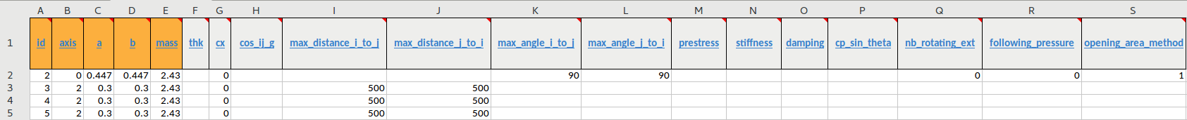
Fig. 8.35 Dynamical Attributes for models A and B
The hinged blowout panel between volumes 1 and 2 (connection #2) has a
vertical rotation axis, from where axis=0. No air drag is taken into
account, therefore cx=0. The flap can open in both directions, from where
max_opening_i_to_j = max_opening_j_to_i=90°. To match as much as possible
[PC16], we deactivate the following pressure
(following_pressure=0).
A3: Sensitivity analysis¶
Once “tuto4” project created (use “isentropic” engine, time step dt=0.00005
and sampling=``0.001, all doors closed) run model A, then model B.
The project page should look like Fig. 8.37.
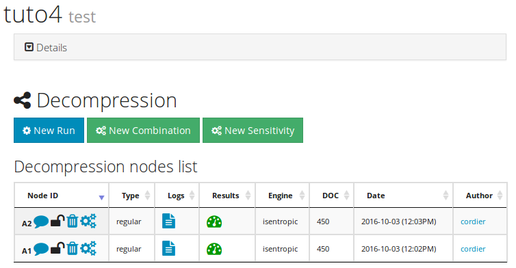
Fig. 8.37 Nodes A1 and A2 before combination
Click on “Sensitivity Analysis” to create node A3. A form (Fig. 8.38) allows you to select reference node (here, select node A1), then all the nodes to be compared (here node A2 only). Then click on “Sensitivity” button to launch the analysis.
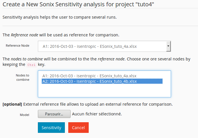
Fig. 8.38 Form to generate a sensitivity Analysis between nodes A1 and A2
Once the run is performed, you are redirected to the newly created A3 node.
The first look should be given to bar graphs and heatmaps available in the “Overview” section. As per regular nodes, overview panels are organized per deck interface (cf. Overview panels).
Main deck to cargo sensitivity¶
The sensitivity to the occupation of the cargo for the floor structure can be checked from the “Main deck to Cargo” data.
Contrary to :ref:pp_heatmap from regular nodes, sensitivity heatmap shows
standard deviation for each pair of load case and interface. The greatest the
value, the greatest the difference.
The heatmap for main deck to cargo interfaces clearly show that having a cargo full or occupied mainly impact Load case 1003, and this for all the interfaces (cf. Fig. 8.39).

Fig. 8.39 Standard deviation for cargo empty or occupied –main dack to cargo interfaces–
Bars graphs will show Δp peaks values for each interface models have in common. If an interface would exist in a model, and not in one of the others, the interface would be omitted.
This graph is handy to check which one of the model is the most critical. Fig. 8.40 clearly shows that occupied cargo is critical for the main deck to cargo interfaces, therefore, for the floor structure.
The X axis is built with each interface of each node (“i/j/Node”): “1/4/A1”, “1/4/A2”, “2/4/A1”, “2/4/A2”, etc.
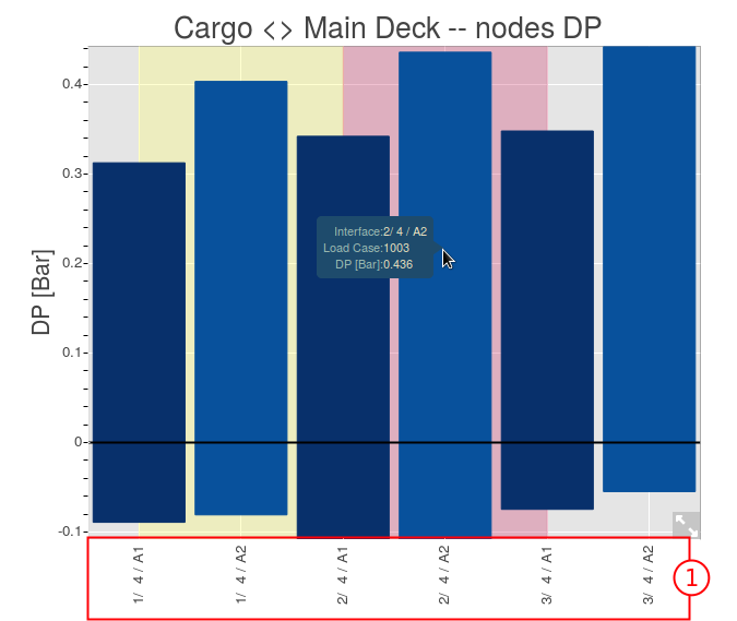
Fig. 8.40 Side by side peaksor cargo empty (A1) or occupied (A2) –main dack to cargo interfaces–
Moving the mouse over the bar graph pops up some tooltips providing some more info about the graph. From those tooltips, all the positive values (from volume x to volume 4, where x is one of {1, 2, 3}) traduce pressure from volume x to volume 4, therefore downward pressures. More over, all the positive values come from load case 1003 (explosion in the Cargo).
Plotting comparative graphs can be done using the dynamic plotter (cf. Fig. 8.41)
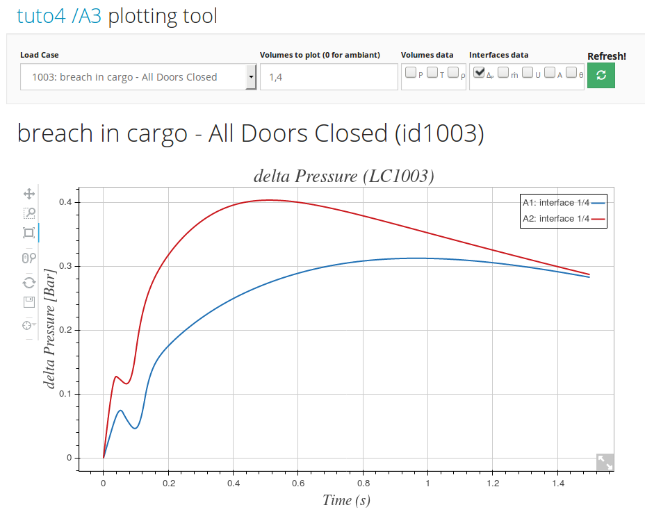
Fig. 8.41 Δp for interface 1/4 and nodes A1 and A2, loadcase 3 (breach in Cargo)
Another way to display detailed decompression information is to use the Layouts tool. If the location of all volumes are properly set up (Volumes deck, sta and rbl of the model) volume and connection info can be displayed on the Aircraft layout at any time of the decompression analysis.
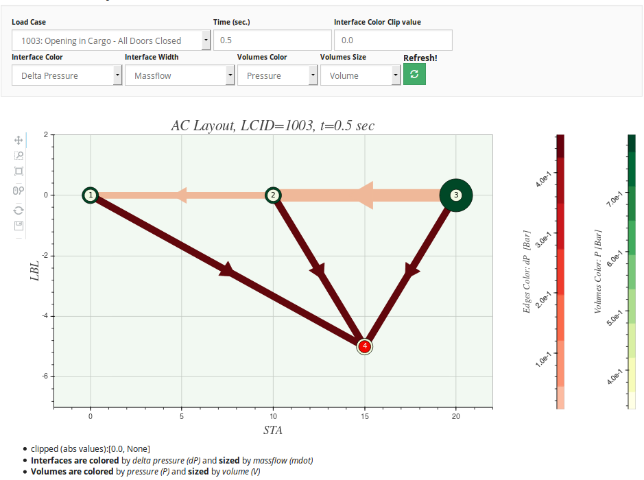
Fig. 8.42 Connection Δp, massflow and volume pressure at t=0.5s (LC1003)
In order to size the cabin, it is not convenient to switch between the two nodes, depending on the interface and the load case. This issue is addressed with Combination Analysis (cf. Combination Analysis for documentation).
A4: Combination¶
From Sensitivity Analysis conducted above, we determined that model A (cargo empty) is critical for explosion in the main deck nad model B (cargo occupied), was critical for an explosion occurring in the cargo.
We will therefore modify models A and B as follows:
- copy ESonix_tuto_4a.xlsx to ESonix_tuto_4c.xlsx, and delete load case #3 (breach in Cargo).
- copy ESonix_tuto_4b.xlsx to ESonix_tuto_4d.xlsx, and delete load case #1 and #2 (breaches in main decks). For demonstration purposes, renumber the remaining load case ID as load case #1.
We now have two models: model A (ESonix_tuto_4c.xlsx) featuring explosion in the main decks with empty cargo, and model B (ESonix_tuto_4d.xlsx) featuring an explosion in the occupied cargo. Run those two models to create respectively Nodes A4 and A5.
Create now a combination analysis (button “New combination” from the project page). The New Combination form is quite similar to the sensitivity’s one. Select Nodes A4 and A5.
This will create the Node A6. Results page for a combination node is very similar to regular run results, although an additional “Combination Load Case Mapping” is provided.
Load case mapping is explained Combination Analysis. The load case mapping for Combination A6 is shown in the result page, panel “Combination Load Case Mapping” (item #2 from Fig. 8.43).
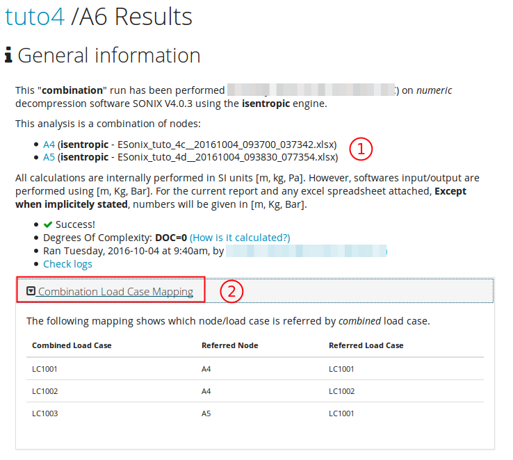
Fig. 8.43 Node A6: Combination results
From the mapping table shown in item #2 from Fig. 8.43, we can see that node A6 has now three load cases (1001, 1002 and 1003), such as
- A6/LC1001 is A4/LC1001 (explosion in entryway with empty cargo)
- A6/LC1002 is A4/LC1002 (explosion in cabin with empty cargo)
- A6/LC1003 is A5/LC1001 (explosion in cargo with occupied cargo)
Tip
Combination Analysis provides the same deliverables, graphs and tools as regular nodes!
With a Combination analysis, we can now check and build a decompression report based on a single set of results, with unique envelop, although two (or more) models are involved in the calculations.
Unified model¶
Combination Analysis is a great step towards a simple yet powerful Aircraft decompression analysis. However, in some cases like the one above, ESonix provides an simpler way to address the multiple models issue: the “Unified Model”.
A Unified Model is a classical ESonix model making use of one, several or all of the following parameters: deor, veor, ovar or exvar.
Those parameters let know to ESonix how to reinitialize the model for each load case.
For the current example, we will use the volume’s veor parameter. “veor” stands for “Volume Explosion Occupation Rate”. By setting Cargo’s veor parameter to 0.6, we let know to ESonix that this volume is reduced by 60% when this volume is the exploded volume.
Copy ESonix_tuto_4a.xlsx to ESonix_tuto_4e.xlsx, and set cargo’s volume definition veor parameter to 0.6 as shown Fig. 8.44, then run a regular analysis on it. This will create the last node of this tutorial: node A7
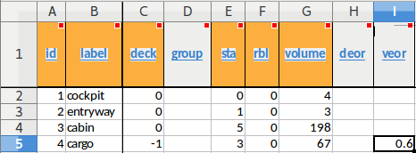
Fig. 8.44 A7 volumes definition
Results for the Unified Model A7 are the same as for the Combination Analysis A6.
Note
To go further
As an exercise, you could now perform an sensitivity Analysis for nodes A6 (Combinated nodes) and A7 (unified model), and check that standard deviation heat maps show really low values.
Downloads¶
You can download the models used through out this tutorial hereunder:
Nodes used to build sensitivity analysis A3:
- node A1 model: http://www.aero-sonix.com/static/support/ESonix_tuto_4a.xlsx
- node A2 model: http://www.aero-sonix.com/static/support/ESonix_tuto_4b.xlsx
Nodes used to build combination analysis A6:
- node A4 model: http://www.aero-sonix.com/static/support/ESonix_tuto_4c.xlsx
- node A5 model: http://www.aero-sonix.com/static/support/ESonix_tuto_4d.xlsx
Unified model Node A7:
- node A7 model: http://www.aero-sonix.com/static/support/ESonix_tuto_4e.xlsx