6. Analysis
ESonix features three kind of analysis:
- Regular
- Combination
- Sensitivity
6.1. Regular runs
Regular runs are the basic analysis in ESonix. Once a project features several regular runs, the user can perform combination or sensitivity analysis on the top of them.
Preparation
A regular run is prepared and run from its father project by clicking on the new
run, button as shown in Fig. 3.4.
The “new run” form is pre-filled with parameters defined during the Project creation (Creating a project).
Basic parameters
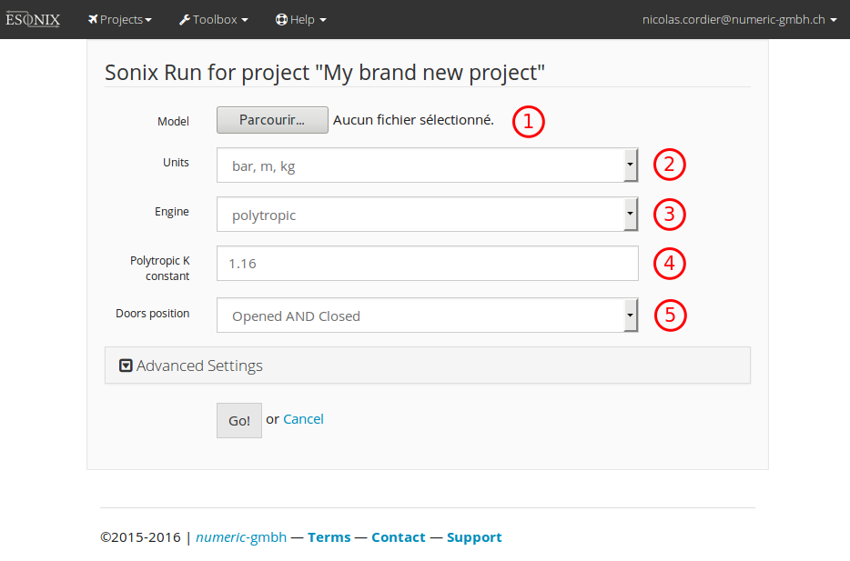
Fig. 6.1 New run basic parameters Form
Basic parameters are (numbers refer to Fig. 6.1):
Model: XLS/XLSX model filename.UnitsSet of units describing the model. SI (modified with bar instead of Pa) or Imperial.Engine: Thermodynamical model (set of equations) to use.Polytropic constant: In casepolytropicengine, or one of its derivative is used, provide the relevant polytropic constant.Door positions: Which initial condition (configuration) to use.
Advanced Parameters
By unfolding the “Advanced parameters” panel, additional parameters are shown:
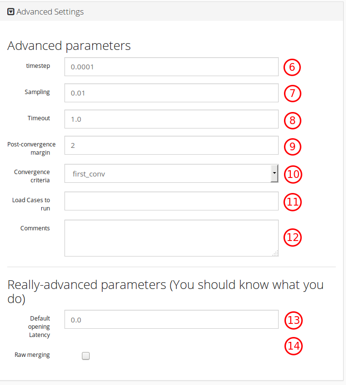
Fig. 6.2 New run advanced parameters Form
Advanced parameters are (numbers refer to Fig. 6.2):
timestep: Simulation time increment.sampling: Data sampling for disk storage.timeout: Simulation maximum time.Post-convergence margin: Margin (in nb of steps) after convergence is reached before stopping calculation.Convergence_criteria: How to calculate convergence. This is a low-influence parameter as most of the time,timeoutwill end the calculation before the real convergence is reached.Load Cases to run: Comma separated list of load cases ID to run. This is useful to restrict calculations to a single or a subset of load cases as defined in the model spreadsheet.Comments: Free text. If blank, ESonix will fill it with miscellaneous data.
Other parameters are for debugging or comparing with OEM data and shouldn’t be tweaked.
Launch and evolution of the run
Once Go! button is pressed, the spreadsheet is sent to the ESonix server,
with the relevant parameters. The spreadsheet is preprocessed and checked. If
it contains no errors, calculation is automatically fired.
6.2. Combination Analysis
Combination analysis provides a mean to combine some regular existing nodes. Combination will build a single set of result based on the provided existing nodes.
To do so, ESonix will begin by creating a load case mapping. This mapping will renumber existing load cases to avoid clash between models. For example, a combination made of three nodes would be mapped as follows:
| combined Load Case | Node ID | LodCase ID |
|---|---|---|
| 1001 | A1 | 1001 |
| 1002 | 1002 | |
| 1003 | 1003 | |
| 1004 | A2 | 1001 |
| 1005 | 1002 | |
| 1006 | A3 | 1001 |
| 1007 | 1018 |
This can be read as follows:
Load Case 1005 for node A4 (combination of A1, A2 and A3) is actually load case 1002 from Node A2.
Once mapping is done, post-processing is performed in the same way as regular runs. All the tools available for regular runs are available for combination nodes, including sensitivity.
Opening in Cabin are usually checked with an empty cargo, such as an important mass of air is available in the cargo to be discharged into the cabin. At opposite, when checking an explosion in the cargo itself, it will be more conservative to assume a cargo occupied. Fig. 6.3 is extracted from Tutorial #4 illustrates the latter example.
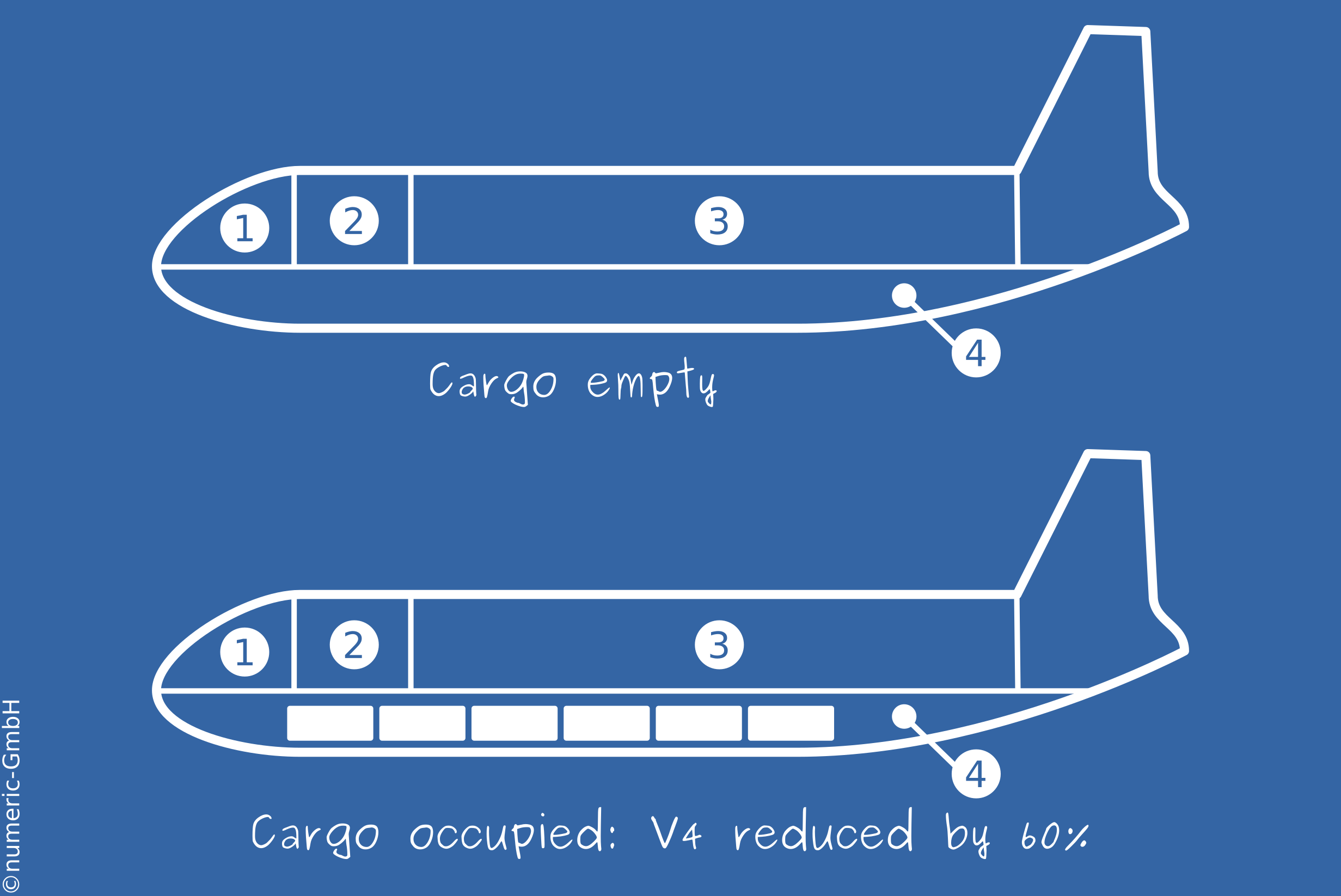
Fig. 6.3 Combination Analysis example
The example illustrated Fig. 6.3 could be addressed by combining two models: one with empty Cargo, one with occupied cargo. The first model would feature load cases for explosions in the main deck only (thus, volumes 1, 2 and 3), while the second one would feature explosion in the cargo (volume 4). The Load Case Mapping would then look like Table 6.2.
| combined Load Case | Node ID | LodCase ID | explosion in |
|---|---|---|---|
| 1001 | A1 | 1001 | vol. 1 |
| 1002 | 1002 | vol. 2 | |
| 1003 | 1003 | vol. 3 | |
| 1004 | A2 | 1001 | vol. 4 |
See also
More details about combination analysis may be found in Tutorial #4.
6.3. Sensitivity Analysis
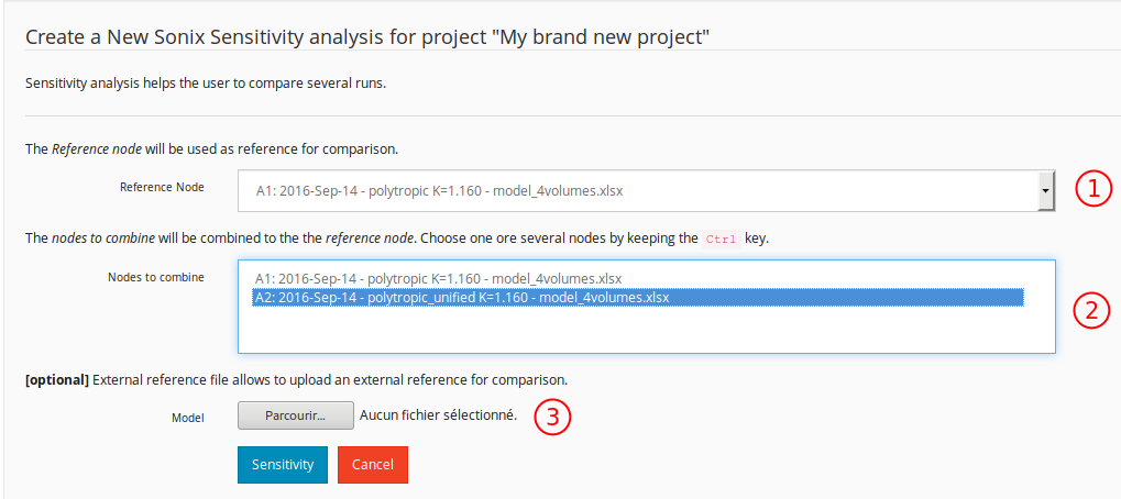
Fig. 6.4 Sensitivity Analysis Form