Overview

What is Nasca?

Nasca is not exactly a software. Nasca aims to be a library providing a complete environment for FEM data processing. Furthermore, a CLI (Command-Line-Interface) and a batch mode are supplied as user interface. Nasca is available for Windows 7 and Unix.

As a library, Nasca proposes to process your data as a flow : you can combine data from a nastran finite elements model, from a database, from user inputs, excel spreadsheets, etc. The process is supposed to lead to the writing of stress-notes, reports, spreadsheets, etc.

Nasca’s dataflow: input/output

NASCA developers target is to release a collection of auto-justificative documents. This excludes a black-box behaviour such as printing list of MS.

Contrariwise, the documents delivered to the engineer are supposed to explain in a maximum extent the way the analysis were performed, such as any checker wouldn’t suspect a software had written it.

Typical input/output data

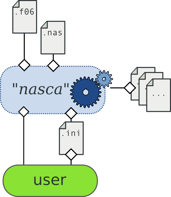
Nasca can read as input files:

• NASTRAN .dat (or .nas, .bdf) models
• NASTRAN .f06 output files. Future release will integrate an additional .op2 reader, but this feature is not supported yet.
• User additional information as a plain -text .ini file.

Outputs files can vary due to the user requests but are typically:

• .neu FEMAP neutral files. This neutral file can be imported in your initial FEM to get the groups collected by Nasca.
• .xlsx Excel 2010 files
• .pdc plain-text files showing literal checks, as if written in the final report. Those files are written using a Markdown syntax (more precisely pandoc-markdown), and can be directly converted to .docx, html, epub, etc. documents by using the wonderful additional pandoc library (cf. [#pandoc]_)

The entry point for a Nasca analysis is the user command known as data processing pipelines. This network of pipelines define the analysis the user wish to run.

Nasca’s architecture

Nasca is mainly written in Python (currently Python 2.7). The migration to Python 3.4 is under process. Besides the python code, some C/C++ code is used for some of the most critical cpu-bound features, such as internal API to NASTRAN files reading.

The Nasca library consists in a core providing a full-featured batteries included API to NASTRAN ASCII files (.dat and .f06). More over, it also provides a powerful yet not sexy interaction with the user via a .ini configuration file.

The core is also coupled to a database (which is currently an on-line PostgreSQL DB, but could be considered as an embedded DB in the future, if this is a customer requirement). This database lets Nasca retrieving on demand allowable on a per-customer basis.

That’s it for the core! No business knowledge is resident in the core. This intended behaviour makes Nasca really flexible and evolutionary by delegating analysis to a plug-in system.

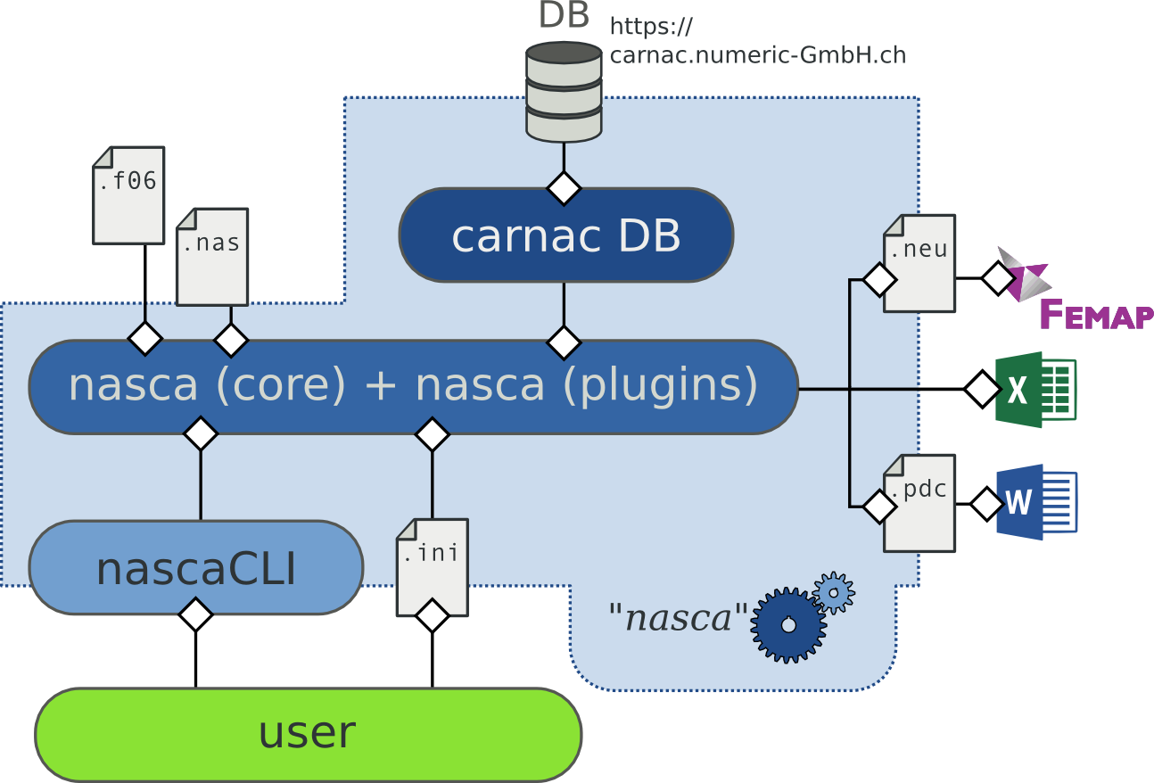
Nasca’s simplified internal dataflow

Data flow processing

Business knowledge and know-how are delegated to plug-ins. Those plug-ins are involved in every step of the data flow analysis. Moreover Each plug-in is a step of this process.

A Nasca analysis can be considered as a set of pipelines driving data through a defined set of steps.

Those steps are incarnated as plugins. Each plug-in can be plugged to the core, but also to other plug-ins in order to build an actual processing pipeline.

For example, a really simple pipeline could be (expressed in pseudo-code):

FEM >> Laminate Panels >> Long Beam Analyse >> Dump output to Excel

To be able to build such a data flow, one needs at least three plug-ins:

Collector

A Collector is in charge of reading the FEM to retrieve the elements and nodes it is in charge of. It can be seen as a grouper that makes group of elements, nodes, etc.

The Collector has the physical and topological knowledge of what is a panel, what is an insert, etc.

Analyst

An analyst can obtain data from a Collector (but from another Analyst as well). Its role is to perform the actual analysis, this means that the MS is calculated at this step. Once the Analyst performed its calculations, it will eventually pipe its data into a Writer.

Writer

The Writer is in charge of post-processing data he may have obtained from an Analyst. It will dump the data into any given format (.xlsx, .pdf, .html, etc.).

A simple pipeline system can be represented as follows (“Take the panels, process their Long Beam, and dump the results”):

Basic analysis pipeline

A fourth type of plug-in exists: the Filter which helps to make analysis a bit more interesting for the engineer by dramatically extending the possibilities.

Filter

The filter steps in the data process to create a fork in a linear analysis.

You could for example imagine to collect all the panels, drive the bulkhead panels to a specialized analyst that takes into account the ribbon direction and dump the results, whereas the panels that are not bulkheads would be driven into the regular analyst. Then you can choose to write the report for all the positive MS and try to save the failing ones by piping them into an alternate analyst. That would lead to the following schematic:

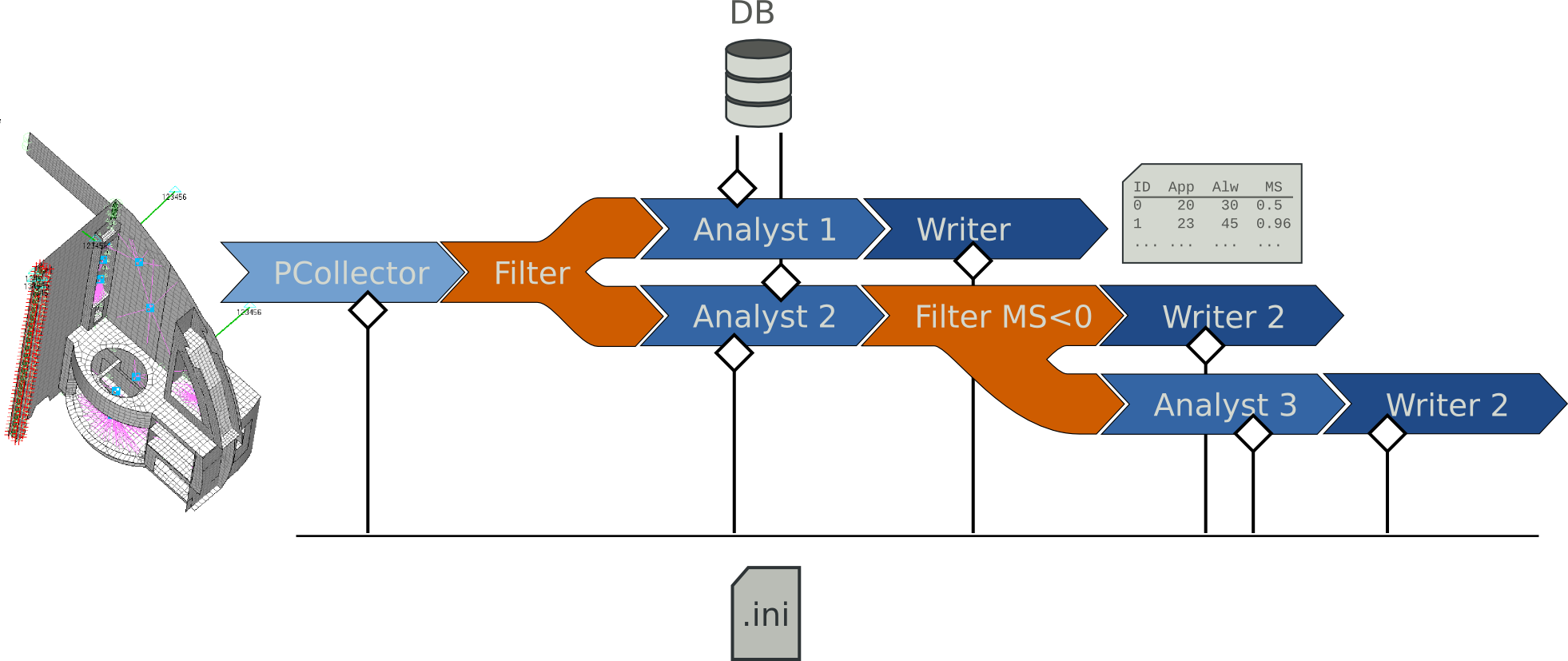
a real-life analysis pipeline

Although this point will be described in a dedicated section, the previous example would be actually written:

C(panels) | IF((TAG=="bulkhead")
              (A(hlcb, ribbon="h") | W(XLS))
              (A(hlcb)  | IF((MS>0)
                                (W(XLS))
                                (A(tsaiwu) | W(XLS))
               )

Tip

A nasca analysis will thus consist in an indeterminate number of pipelines

A powerful user input: the .ini file

Nasca Collectors can retrieve a lot of features from a simple FEM. Simply consider CBUSH: a CBUSH can be used to idealize many features: Floor attachments, bulkhead fittings, inserts, etc... But, how does the insert can collect only the relevant elements?

Actually, the Collector “inserts” will search elements matching a certain set of constraints. The following options are the default ones used to search inserts:

max_length = 1.0
min_length = 0.0
shall_be_grounded = False
shall_not_be_grounded = False
shall_be_in_plane = False
shall_not_be_in_plane = False
### z_range: list of two integers
# set the z range allowed for items. Otherwise discarded
z_range = 2.0, 2000.0
###  prop_black_list: list of strings.
# if one of this string is detected in the FEMAP property, the item
# will be discarded
prop_black_list = bracket, pallet, dummy, insert, attach, upper
### connected_panel_position: position.
# choice: {"any", "horizontal" | "vertical" | "not_horizontal" |
#          "not_vertical" | "any"}
connected_panel_position = any

When running Nasca for the first time over a model, Nasca will create this configuration files, and dumps into all the default options. By this way, the user just has to modify the options he needs.

FEMAP feedback: the neutral file

During the grouping phase when are triggered all the requested collectors, Nasca creates a feeds a Femap neutral file (.neu). This file contains all the groups created during the analysis.

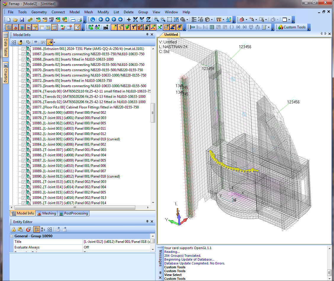
Femap groups after Nasca’s neutral import

All the documents can thus refer to any item (e.g. Panel 07, T-Joint 123, etc.). This is a convenient and human way to automatize reporting: any checker can then easily refer to the FEM to cross-check Nasca’s output.

Besides this asset, it also provides a convenient way to specify some non-default options in the configuration file.

Nasca deliveries

Nasca can deliver several files during an anlysis. Some of them are mandatory, whereas some of them are optional and choosen either via some options to activate, either via the pipelines command.

Mandatory outputs

The log files generated during the analysis.

Optional outputs

Depending on the Writer plug-ins activated, one can get several outputs:

• .xlsx as native Excel Files
• .pdc pandoc-Markdown plain-text files.

The pandoc-markdown plain-text files

This format has been chosen by the developers of Nasca as default output format. The following Pros were taken into considerations:

• plain-text file: no need of extra software to open it; the default windows notepad can open it, although some more convenient text editors will be definitely more comfortable (e.g. Notepad++ [1]).
• human super-easy reading: Its syntax is immediately understandable. No need to convert it to read it.
• easily editable, to complete or detail the report.
• convertible to any of the following formats: HTML, LaTeX, PDF, Microsoft Word docx. This requires the use of the excellent open-source pandoc [#pandoc]_ software (available for windows and Unix).
• Excellent handling of equations by using the scientific standard: latex. Once rendered in Word, they will become native Microsoft equations.

Example of rendering (from Nasca 0):

###  Blkh Floor Fitting fitted in NL610-10633-1000 ###

Those results are visible from the Femap model group id11066 named *[bulkhead floor fit. 01] Blkh Floor Fitting fitted in NL610-10633-1000*.

**Allowable**

      Part Ref.             Panel Ref       Long. Shear   Trans. Shear    Tension
----------------------- ------------------ ------------- -------------- -----------
Fitting                  nl610-10633-1000   3473          1806           4857
Std. Adaptor Block       *n.a.*             2782.0        2920.0         2877.0
**Combined Allowable**   *n.a.*             **2782.0**    **1806.0**     **2877.0**

**Envelop Results**

 eid    lc     fx       fy       fz     Long.   Trans.   Tension    MS
------ ---- -------- -------- -------- ------- -------- --------- ------
12307   2    -10.11   -12.75   394.83   12.7    -10.1    394.8     +6.28
12308   2    -26.27   -13.26   952.87   13.3    -26.3    952.9     +2.02

**Critical MS**

$MS_{Blkh\ Floor\ Fitting,\ LC2} = \frac{1}{\sqrt{{\frac{13.30}{2782.00}}^2+{\frac{-26.30}{1806.00}}^2+{\frac{952.90}{2877.00}}^2}}-1=+2.02$

Once rendered to PDF:

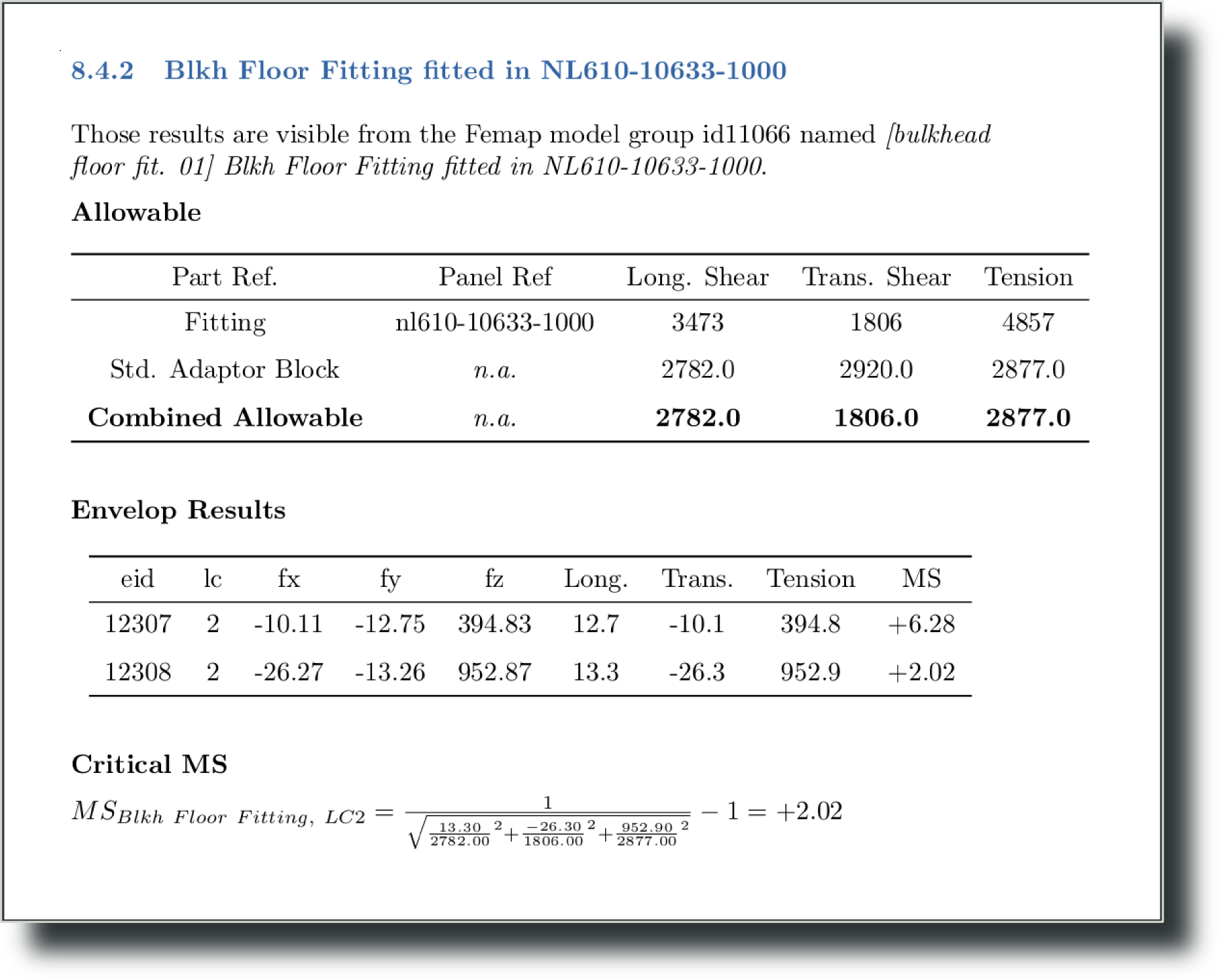
pandoc rendering to PDF

Footnotes

[1]	Free open-source text editor for windows: http://www.notepad-plus-plus.org/